Estimation Risk and Shrinkage

Every portfolio in Portfolios of Risky Assets, Beta Pricing and The Treynor-Black Model was built from expected returns and covariances that the investor knows. In practice they are estimated from data, and the estimates are noisy. An optimizer cannot tell estimation error from opportunity: it puts the largest weights on the assets whose estimated means are highest and whose estimated risks are lowest, which are often the assets whose estimates are most wrong. This chapter measures how large the errors are, shows what they do to the portfolios of the earlier chapters, and develops the main remedy, shrinkage: pulling the estimates toward a simpler structure that is wrong in detail but much less noisy.

Means and Variances from Data

Suppose returns are independent over time, with an annual expected return \mu and volatility \sigma, and we observe Y years of data at n equally spaced dates. Merton (1980) pointed out that the two parameters are learned in very different ways. The average continuously compounded return over the whole period depends only on the first and last prices, so sampling more often does not help: the standard error of the estimated annual mean depends only on the calendar length of the sample. The volatility, on the other hand, is estimated more precisely the more often we sample. For approximately normal returns, \text{SE}(\hat{\mu}) = \frac{\sigma}{\sqrt{Y}} \qquad \text{SE}(\hat{\sigma}) \approx \frac{\sigma}{\sqrt{2 n}}. \tag{1}

Merton, Robert C. 1980. “On Estimating the Expected Return on the Market: An Exploratory Investigation.” Journal of Financial Economics 8 (4): 323–61.

Example 1 (How Well Do We Know the Market?) The U.S. market portfolio earned an average excess return of 8.3% a year from July 1926 to December 2025, with a volatility of 18.4%. By (1), 100 years of data give a standard error of 1.84% for the risk premium, while the 1,194 monthly returns give a standard error of 0.38% for the volatility. With only ten years of monthly data, the standard error is 5.8% for the premium, larger than the premium itself, and 1.2% for the volatility. To estimate the premium within one percentage point with 95% confidence, we would need (1.96 \times 0.18 / 0.01)^{2} \approx 1,299 years of data.

Covariances behave like variances, so they are estimated well from monthly or daily data, at least one at a time. The difficulty with covariances is their number: N assets have N (N + 1) / 2 variances and covariances, as the counting exercise in The Index Model showed. Expected returns are few, N of them, but each one is hard to estimate. Mean-variance optimization needs both.

The Plug-In Portfolio

The tangency portfolio of Beta Pricing has weights proportional to \pmb{\Sigma}^{-1} \pmb{\mu}, where \pmb{\mu} is the vector of expected excess returns and \pmb{\Sigma} the covariance matrix. Its squared Sharpe ratio is \pmb{\mu}^{\top} \pmb{\Sigma}^{-1} \pmb{\mu}. The plug-in portfolio replaces \pmb{\mu} and \pmb{\Sigma} with their sample estimates \hat{\pmb{\mu}} and \hat{\pmb{\Sigma}} from T months of data. In the sample used to estimate it, the plug-in portfolio has the highest Sharpe ratio of any portfolio, by construction, and that is the problem. It fits the noise in the sample means as well as the true premia. Even if every asset had a true expected excess return of zero and \pmb{\Sigma} were known, the sample mean would be \hat{\pmb{\mu}} \sim N(\mathbf{0}, \pmb{\Sigma} / T), and the in-sample squared monthly Sharpe ratio \hat{\pmb{\mu}}^{\top} \pmb{\Sigma}^{-1} \hat{\pmb{\mu}} would average N / T. The more assets per month of data, the more spurious the in-sample performance.

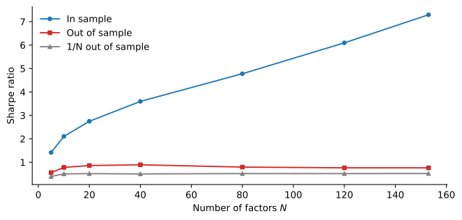
The factors of Jensen et al. (2023), which Beyond the CAPM used to describe the factor zoo, make the point. We estimate the plug-in portfolio from 1972 to 1998, T = 324 months, and hold it from 1999 to 2025. Figure 1 shows its Sharpe ratio in both periods for random sets of N factors. In sample, the Sharpe ratio rises steadily as factors are added, to 7.3 with all 153 factors. With N / T = 0.47, noise alone would produce an annualized Sharpe ratio of about \sqrt{12 \times 0.47} = 2.4 if the covariance matrix were known, and about 3.3 with it estimated, as here. The in-sample Sharpe ratio is well above both, so the factors carry real premia, but little of the in-sample fit survives. Out of sample, the Sharpe ratio peaks at 0.89 with 40 factors and falls to 0.76 with all of them. The equally weighted portfolio of the same factors earns about 0.50, close to the market’s 0.50.

Jensen, Theis Ingerslev, Bryan Kelly, and Lasse Heje Pedersen. 2023. “Is There a Replication Crisis in Finance?” The Journal of Finance 78 (5): 2465–518.

Figure 1: Annualized Sharpe ratio of the plug-in tangency portfolio of N JKP factors, estimated from 1972 to 1998, in that period and from 1999 to 2025, and of the equally weighted portfolio of the same factors from 1999 to 2025. Each point averages 50 random sets of factors, except the last, which uses all of them.

The JKP factors have large premia, so among them estimating the means still pays something. The period after 1998 is out of sample only for the estimation, though. Many of the factors were discovered with data from that period, as The Factor Zoo in Real Time shows, and the Sharpe ratios here and below are before trading costs, which What Do Anomalies Cost to Trade? measures. Among individual stocks or broad asset classes the premia are smaller relative to their noise, and the plug-in portfolio does worse. DeMiguel et al. (2009) compared the plug-in portfolio and 13 extensions designed to reduce estimation error with the naive rule that puts 1/N of wealth in each asset. Across seven data sets, none of the 14 models was consistently better than 1/N out of sample in Sharpe ratio, certainty-equivalent return or turnover. With parameters calibrated to U.S. stocks, the plug-in portfolio needs an estimation window of about 3,000 months to beat 1/N with 25 assets, and about 6,000 months with 50. Kan and Zhou (2007) show that estimation risk also breaks the two-fund separation of The CAPM: an investor who knows that the inputs are estimated does better by combining the sample tangency portfolio with the sample minimum-variance portfolio, which does not depend on the noisy means, than by holding the sample tangency portfolio alone.

DeMiguel, Victor, Lorenzo Garlappi, and Raman Uppal. 2009. “Optimal Versus Naive Diversification: How Inefficient Is the 1/N Portfolio Strategy?” Review of Financial Studies 22 (5): 1915–53.

Kan, Raymond, and Guofu Zhou. 2007. “Optimal Portfolio Choice with Parameter Uncertainty.” Journal of Financial and Quantitative Analysis 42 (3): 621–56.

Shrinking the Covariance Matrix

The minimum-variance portfolio of Portfolios of Risky Assets avoids expected returns altogether, so it isolates the problem of estimating \pmb{\Sigma}. Each covariance is estimated well, but there are many of them, and the optimizer combines them. When N is not small relative to T, the sample covariance matrix \hat{\pmb{\Sigma}} contains some extreme entries, extreme not because they are right but because they have the most error, and the optimizer places its largest bets on them. With N \geq T the sample matrix cannot even be inverted. There are three common remedies.

Impose a structure. The Index Model implies that the covariance between two stocks is \beta_{i} \beta_{j} \sigma_{M}^{2}. In matrix form, the single-index (SI) covariance matrix is \pmb{\Sigma}_{\text{SI}} = \sigma_{M}^{2} \pmb{\beta} \pmb{\beta}^{\top} + \mathbf{D}, \tag{2} where \mathbf{D} is the diagonal matrix of the firm-specific variances \sigma^{2}(e_{i}). The estimate needs 2 N + 1 parameters instead of N (N + 1) / 2. Its error is that it ignores industry and other common factors, which the sample matrix captures.

Shrink toward the structure. The sample matrix \hat{\pmb{\Sigma}} is unbiased but noisy, and a structured matrix is biased but precise. Ledoit and Wolf (2004) propose a weighted average of the two, \hat{\pmb{\Sigma}}_{\delta} = \delta \pmb{\Sigma}_{\text{CC}} + (1 - \delta) \hat{\pmb{\Sigma}}, \qquad 0 \leq \delta \leq 1, \tag{3} where the target \pmb{\Sigma}_{\text{CC}} is the constant-correlation (CC) matrix, which keeps each sample variance and sets every correlation to the average sample correlation. The shrinkage intensity \delta is chosen from the data to minimize the expected squared distance between \hat{\pmb{\Sigma}}_{\delta} and the true \pmb{\Sigma}. The single-index matrix \pmb{\Sigma}_{\text{SI}} (2) can take the place of \pmb{\Sigma}_{\text{CC}} as the target, and Ledoit and Wolf report that the two perform about the same. The optimal \delta is larger when the sample matrix is noisier, with fewer months of data, and smaller when the target is far from the true matrix, a distance estimated by how far the target is from the sample matrix.

Ledoit, Olivier, and Michael Wolf. 2004. “Honey, i Shrunk the Sample Covariance Matrix.” Journal of Portfolio Management 30 (4): 110–19.

Jagannathan, Ravi, and Tongshu Ma. 2003. “Risk Reduction in Large Portfolios: Why Imposing the Wrong Constraints Helps.” Journal of Finance 58 (4): 1651–83.

Rule out short sales. Forbidding short sales removes the long-short positions that depend on the directions the data cannot pin down. When N \geq T the sample matrix is singular and the unconstrained minimum-variance portfolio does not exist, but the constrained one does. When the sample matrix is invertible, Jagannathan and Ma (2003) show that the constraint is equivalent to shrinking the largest covariance estimates, and they find that once short sales are ruled out, the sample covariance matrix performs about as well as estimates based on factor models, shrinkage estimators and daily data.

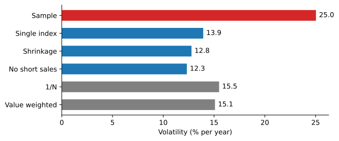
Figure 2 compares the remedies out of sample. Each January from 1972 to 2025, we take the 100 largest U.S. stocks that have returns in each of the previous 120 months, estimate the covariance matrix from those months, and hold the minimum-variance portfolio for the year. With only 120 months for 100 stocks, the sample matrix is invertible but noisy, and the portfolio built from it has a volatility of 25.0%, far above the 15.1% of the value-weighted portfolio of the same stocks. The single-index matrix brings the volatility down to 13.9%, shrinkage to 12.8%, with an average intensity \delta of 0.50, and the sample matrix with no short sales to 12.3%. All three are below the 15.5% of the equally weighted portfolio. For covariances, disciplined estimation pays reliably. For means, it pays only when the premia are large relative to their noise, as among the JKP factors.

Figure 2: Annualized volatility of minimum-variance portfolios of the 100 largest U.S. stocks, re-estimated each January from the previous 120 months and held for a year, 1972 to 2025, with four estimates of the covariance matrix, and of the equally weighted and value-weighted portfolios of the same stocks.

Shrinking Expected Returns

Shrinkage works for expected returns too, and since means are estimated much less precisely than covariances, it matters even more. The question is what to shrink toward.

Black-Litterman

Black and Litterman (1992) observed that mean-variance optimizers fed with an investor’s estimates of expected returns produce extreme portfolios that the investor would never hold, because the portfolio is extremely sensitive to the expected returns, and that small changes in the inputs move the weights wildly. Their solution is to start from the expected returns that would make the market portfolio optimal. If an investor with risk aversion A holds the market, the first-order condition of mean-variance utility, \mathbf{w}_{M} = (A \pmb{\Sigma})^{-1} \pmb{\pi}, can be inverted to give the equilibrium risk premiums \pmb{\pi} = A \pmb{\Sigma} \mathbf{w}_{M}. \tag{4} These are the premiums of the CAPM, since \pmb{\Sigma} \mathbf{w}_{M} is the vector of covariances of each asset with the market. They are a neutral starting point: an investor with no views holds the market.

Black, Fischer, and Robert Litterman. 1992. “Global Portfolio Optimization.” Financial Analysts Journal 48 (5): 28–43.

The investor then states views, as many or as few as they have, each with a degree of confidence. In the Black-Litterman model, the prior is that \pmb{\mu} is centered on \pmb{\pi} with covariance matrix \tau \pmb{\Sigma}, where the scalar \tau measures how uncertain the equilibrium premiums are. A view says that a portfolio \mathbf{p}, which can be long-short, has an expected excess return of q, with a variance \omega that measures the investor’s lack of confidence. Combining the prior and the view as two noisy signals gives \pmb{\mu}_{\text{BL}} = \pmb{\pi} + \tau \pmb{\Sigma} \mathbf{p} \, \frac{q - \mathbf{p}^{\top} \pmb{\pi}}{\tau \mathbf{p}^{\top} \pmb{\Sigma} \mathbf{p} + \omega} \qquad \mathbf{w}_{\text{BL}} = \mathbf{w}_{M} + \mathbf{p} \, \frac{\tau (q - \mathbf{p}^{\top} \pmb{\pi})}{A (\tau \mathbf{p}^{\top} \pmb{\Sigma} \mathbf{p} + \omega)}. \tag{5} The first equation moves every asset’s expected return in proportion to its covariance with the view portfolio, by the amount the view differs from equilibrium, scaled down by the uncertainty of the view. The second follows from \mathbf{w} = (A \pmb{\Sigma})^{-1} \pmb{\mu}_{\text{BL}}: the investor holds the market plus a position in the view portfolio, much as the Treynor-Black investor holds the market plus an active portfolio. With no confidence in the view, \omega \to \infty, the investor holds the market. With full confidence, \omega = 0, the expected return of \mathbf{p} equals q.

Example 2 (A Relative View) A market has two assets, U.S. and international stocks, with volatilities of 20% and 15%, a correlation of 0.5, and market weights of 60% and 40%. With A = 2.5, (4) gives \pmb{\Sigma} \mathbf{w}_{M} = \begin{pmatrix} 0.04 & 0.015 \\ 0.015 & 0.0225 \end{pmatrix} \begin{pmatrix} 0.6 \\ 0.4 \end{pmatrix} = \begin{pmatrix} 0.030 \\ 0.018 \end{pmatrix} \qquad \pmb{\pi} = 2.5 \times \begin{pmatrix} 0.030 \\ 0.018 \end{pmatrix} = \begin{pmatrix} 7.5\% \\ 4.5\% \end{pmatrix}. An investor believes that U.S. stocks will outperform international stocks by 5%, against the 3% of equilibrium, so \mathbf{p} = (1, -1)^{\top} and q = 0.05. The view portfolio has variance \mathbf{p}^{\top} \pmb{\Sigma} \mathbf{p} = 0.04 + 0.0225 - 2 \times 0.015 = 0.0325 and covariances \pmb{\Sigma} \mathbf{p} = (0.025, -0.0075)^{\top} with the two assets. With \tau = 0.05 and a view as uncertain as the prior, \omega = \tau \mathbf{p}^{\top} \pmb{\Sigma} \mathbf{p} = 0.001625, the scaling factor in (5) is 0.05 \times 0.02 / 0.00325 = 0.3077, so \pmb{\mu}_{\text{BL}} = \begin{pmatrix} 7.5\% \\ 4.5\% \end{pmatrix} + 0.3077 \begin{pmatrix} 0.025 \\ -0.0075 \end{pmatrix} = \begin{pmatrix} 8.27\% \\ 4.27\% \end{pmatrix} \qquad \mathbf{w}_{\text{BL}} = \begin{pmatrix} 0.6 \\ 0.4 \end{pmatrix} + \frac{0.3077}{2.5} \begin{pmatrix} 1 \\ -1 \end{pmatrix} = \begin{pmatrix} 72.3\% \\ 27.7\% \end{pmatrix}. The expected outperformance is 4%, halfway between equilibrium and the view, because the investor trusts the two equally. The portfolio tilts 12.3 percentage points toward U.S. stocks and is otherwise the market.

Ridge and Principal Components

Black-Litterman needs views. Without them, we can still ask which estimated means deserve the least trust. Write the covariance matrix in terms of its eigenvalues \lambda_{j} and eigenvectors \mathbf{v}_{j}. Each eigenvector is a portfolio, a principal component of the assets, with variance \lambda_{j}, and the components are uncorrelated. The tangency weights split into one position per component, \pmb{\Sigma}^{-1} \pmb{\mu} = \sum_{j=1}^{N} \mathbf{v}_{j} \, \frac{\mathbf{v}_{j}^{\top} \pmb{\mu}}{\lambda_{j}}, \tag{6} where \mathbf{v}_{j}^{\top} \pmb{\mu} is the expected return of component j. The components with the smallest variance get the largest weights. With estimated inputs, those are exactly the components whose estimated means are mostly noise, since a small sample mean divided by a tiny variance is a huge position.

Kozak et al. (2020) argue on economic grounds that a low-variance component should not have a high Sharpe ratio: a near-riskless portfolio with a large expected return is a near-arbitrage that arbitrageurs would trade away. This prior implies shrinking the weights of low-variance components the most, which leads to the ridge estimator \mathbf{w}_{\gamma} = (\hat{\pmb{\Sigma}} + \gamma \mathbf{I})^{-1} \hat{\pmb{\mu}} = \sum_{j=1}^{N} \mathbf{v}_{j} \, \frac{\mathbf{v}_{j}^{\top} \hat{\pmb{\mu}}}{\lambda_{j} + \gamma}. \tag{7} Adding the same \gamma to every eigenvalue barely changes the position in a high-variance component and cuts the position in a low-variance one sharply. The plug-in portfolio is the case \gamma = 0.

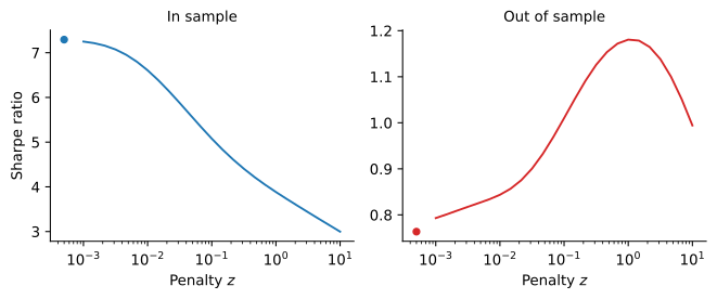
Figure 3 applies (7) to all 153 factors, with the same estimation and evaluation periods as Figure 1. The penalty is \gamma = z \bar{\lambda}, a multiple z of the average eigenvalue. As z rises, the in-sample Sharpe ratio falls, from 7.3 for the plug-in portfolio to 3.9 at z = 1, while the out-of-sample Sharpe ratio rises from 0.76 to 1.18. Shrinkage gives up fit in the sample to gain performance outside it. The peak uses the z that did best from 1999 to 2025, which an investor in 1998 could not know, so it overstates what ridge delivers in real time. Every penalty from z = 0.1 to z = 10 earns at least 0.99, though, so the gain over the plug-in portfolio does not depend on a lucky choice. Choosing z each month from past data gives up little of it in An SDF for the Factor Zoo, but The Factor Zoo in Real Time shows that the same rule can fail when the menu holds only the factors known at the time. With too much shrinkage, the weights become proportional to the sample means, and the out-of-sample Sharpe ratio starts falling again.

Figure 3: Annualized Sharpe ratio of the ridge portfolio of all JKP factors, estimated from 1972 to 1998, in that period and from 1999 to 2025, against the penalty z as a multiple of the average eigenvalue. The points at the left are the plug-in portfolio, z = 0.

How Many Factors?

Shrinkage also bears on the second question of the factor zoo, how many factors a model needs. The ridge portfolio keeps every component, so to answer it Kozak et al. (2020) add a second penalty, on the absolute size of the weights, which sets some of them to zero. They find that models built from a few characteristic-based factors, like the four- and five-factor models, cannot adequately summarize the cross-section of expected returns, while a small number of principal components can. Lettau and Pelger (2020) extend principal component analysis with a penalty on pricing errors and find five factors with economic meaning. Kelly et al. (2019) let characteristics determine each stock’s time-varying factor loadings, and find that five such latent factors explain average returns better than existing models, with small and insignificant anomaly intercepts. Feng et al. (2020) propose a test of whether a new factor adds to a high-dimensional set of existing ones, and find that most recently proposed factors are redundant, though a few are not. The common thread is that a few well-chosen combinations of characteristics capture much more than a short list of individual anomaly factors. How few is less settled. In Is There an Eigenvalue Cliff?, five principal components of the JKP factors earn an out-of-sample Sharpe ratio of about 1.1, against about 1.9 for the ridge portfolio of all of them, and they need 20 to 30 components to catch up.

Kozak, Serhiy, Stefan Nagel, and Shrihari Santosh. 2020. “Shrinking the Cross-Section.” Journal of Financial Economics 135 (2): 271–92.

Lettau, Martin, and Markus Pelger. 2020. “Factors That Fit the Time Series and Cross-Section of Stock Returns.” Review of Financial Studies 33 (5): 2274–325.

Kelly, Bryan T., Seth Pruitt, and Yinan Su. 2019. “Characteristics Are Covariances: A Unified Model of Risk and Return.” Journal of Financial Economics 134 (3): 501–24.

Feng, Guanhao, Stefano Giglio, and Dacheng Xiu. 2020. “Taming the Factor Zoo: A Test of New Factors.” Journal of Finance 75 (3): 1327–70.

Complexity

The lesson so far is that a model with too many parameters for the data overfits, and that shrinkage helps. Recent work in machine learning finds a surprise when the number of parameters grows past the number of observations. With N > T, the sample covariance matrix is singular, many portfolios fit the sample perfectly, and the ridgeless portfolio is the limit of (7) as \gamma \to 0, the one among them with the smallest weights. Its out-of-sample performance is poor when N is close to T, where the smallest nonzero eigenvalues are close to zero and (6) puts huge weights on noise, but it recovers as N grows past T. Hastie et al. (2022) study this “double descent” in ridgeless regression.

Hastie, Trevor, Andrea Montanari, Saharon Rosset, and Ryan J. Tibshirani. 2022. “Surprises in High-Dimensional Ridgeless Least Squares Interpolation.” The Annals of Statistics 50 (2): 949–86.

Kelly, Bryan, Semyon Malamud, and Kangying Zhou. 2024. “The Virtue of Complexity in Return Prediction.” The Journal of Finance 79 (1): 459–503.

Didisheim, Antoine, Shikun Barry Ke, Bryan T. Kelly, and Semyon Malamud. 2023. Complexity in Factor Pricing Models. Working Paper No. 31689. National Bureau of Economic Research.

Kelly et al. (2024) call it the virtue of complexity. They predict the return of the U.S. market from 15 standard predictors, such as the dividend yield and the term spread, with models that range from one parameter to more than 10,000, estimated from as few as 12 months of data, and use the predictions to time the market. From 1926 to 2020, the out-of-sample Sharpe ratio of their timing strategies exceeds that of the market by up to about 0.47 a year, even though the out-of-sample R^{2} of most of the models is substantially negative. Here the negative R^{2} comes from forecasts that are too volatile, not from forecasts that point the wrong way, and a timing strategy can profit from forecasts that are correlated with the truth even when their scale is off. Didisheim et al. (2023) find the same pattern in the cross-section, where SDFs with more factors than observations outperform simpler ones by a large margin.

The result is debated. Nagel (2025) shows that with 12 months of training data and thousands of parameters, the forecast reduces to a weighted average of the last 12 returns, with the largest weights on the most recent months and larger weights when the predictors are calm: a volatility-timed momentum strategy. On artificial returns that reverse instead of continuing, the method builds the same strategy and loses money, so in his reading it does not learn from the data, and its historical success is a coincidence. Kelly and Malamud (2025) reply that predictors simulated with the same persistence but unrelated to returns produce almost no predictability, and that the same patterns appear with long training samples. The disagreement is about how much can be learned from very short samples. Nagel agrees that a large model can beat a small, misspecified one.

Nagel, Stefan. 2025. Seemingly Virtuous Complexity in Return Prediction. Working Paper No. 34104. National Bureau of Economic Research.

Kelly, Bryan, and Semyon Malamud. 2025. Understanding the Virtue of Complexity. Working Paper No. 5346842. SSRN.

Figure 4 repeats the experiment with the JKP factors. Each month from January 1977, we estimate the ridgeless and ridge portfolios of N randomly chosen factors from the previous T = 60 months, scale the weights so that their absolute values sum to one, and hold the portfolio for a month. The ridgeless Sharpe ratio rises with N at first, collapses to 0.32 near N = T, and recovers to 1.25 with all 153 factors, more than twice as many parameters as observations. With a small penalty, z = 0.1, the collapse disappears. The Sharpe ratio rises with N to 1.73 at N = T and changes little after that, reaching 1.75 with all the factors.

Figure 4: Annualized out-of-sample Sharpe ratio of ridgeless and ridge (z = 0.1) portfolios of N JKP factors, re-estimated each month from the previous 60 months, against the complexity N / T. Each point averages five random sets of factors, except the last, which uses all of them. The dashed line marks N = T.

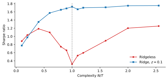
The figure shows the double descent of the ridgeless portfolio but gives only weak support to the virtue of complexity: with all the factors, its Sharpe ratio of 1.25 is barely above the 1.19 of the best ridgeless portfolio with fewer factors than months. It also shows where the recovery comes from. Once N > T, the minimum-norm solution ignores the directions that the data cannot see and spreads its weights across many factors, which is a form of shrinkage, and the more factors there are, the more it shrinks. An explicit penalty does the same job better: the ridge portfolio beats the ridgeless one at every N beyond a handful of factors. Many parameters do not hurt when they are shrunk, and the protection against overfitting is the shrinkage, not a small model.

This experiment differs from the ones in the debate. It combines 153 published factors rather than random nonlinear transformations of a few predictors or characteristics, and it trains on five years of data rather than one, so it says nothing about Nagel’s point on 12-month windows. An SDF for the Factor Zoo runs the same test with more windows and finds the same pattern. Within it, the evidence sides with neither strong claim: without shrinkage, complexity barely pays, and with shrinkage, parameters beyond N = T stop hurting but help little. The notebooks Implementing the Minimum-Variance Portfolio and An SDF for the Factor Zoo in From Papers to Portfolios carry these estimates further, with daily data, longer windows and penalties chosen from past data.

Practice Problems

These problems give you a chance to practice the concepts introduced in this chapter. Try to solve each one on your own before expanding the solution.

Problem 1 (A Ten-Year Track Record) A fund has ten years of monthly returns, with an average excess return of 6% a year and a volatility of 18%.

1. What is the standard error of the estimated annual mean? Is the mean significantly different from zero at the 5% level?
2. What is the approximate standard error of the estimated volatility?
3. Would daily data for the same ten years improve either estimate?
4. How many years of data would make an average excess return of 6% significant at the 5% level, if the volatility stays at 18%?

Solution

1. By (1), \text{SE}(\hat{\mu}) = 0.18 / \sqrt{10} = 5.69\%. The t-statistic is 6 / 5.69 = 1.05, well below 1.96, so the mean is not significantly different from zero.

2. With n = 120, \text{SE}(\hat{\sigma}) \approx 0.18 / \sqrt{240} = 1.16\%.

3. Daily data, about 2,520 observations, would cut the standard error of the volatility to about 0.18 / \sqrt{5{,}040} = 0.25\%. The standard error of the mean would not change, since it depends only on the ten years.

4. We need 0.06 / (0.18 / \sqrt{Y}) \geq 1.96, or Y \geq (1.96 \times 0.18 / 0.06)^{2} = 34.6 years.

Problem 2 (Sharpe Ratios from Noise) An analyst estimates the plug-in tangency portfolio of 50 strategies from 120 months of returns. Unknown to the analyst, every strategy has a true expected excess return of zero.

1. What in-sample monthly squared Sharpe ratio should the analyst expect, if the covariance matrix were known? What annualized Sharpe ratio does it correspond to?
2. What Sharpe ratio should the analyst expect out of sample?
3. How does the in-sample Sharpe ratio change with 500 months of data?

Solution

1. The expected squared monthly Sharpe ratio is N / T = 50 / 120 = 0.417, a monthly Sharpe ratio of \sqrt{0.417} = 0.645 and an annualized one of 0.645 \times \sqrt{12} = 2.24. With an estimated covariance matrix it would be higher still.

2. Zero. The portfolio’s weights depend only on past noise, and every strategy has an expected excess return of zero in the future, so any portfolio of them does too.

3. N / T = 50 / 500 = 0.1, so the annualized in-sample Sharpe ratio falls to \sqrt{0.1 \times 12} = 1.10. More data reduce the spurious performance, but slowly, with the square root of T.

Problem 3 (Shrinking a Correlation) Two stocks have volatilities of 30% and 20%. Their sample correlation is 0.9, while the single-index model, with betas of 1.2 and 0.8 and a market volatility of 20%, implies a covariance of 1.2 \times 0.8 \times 0.04 = 0.0384, a correlation of 0.64. Suppose the single-index covariance is the true one.

1. Find the minimum-variance weights from the sample covariance and their true volatility.
2. Repeat with the covariance shrunk halfway toward the single-index model, \delta = 0.5 in (3) with \pmb{\Sigma}_{\text{SI}} as the target, keeping the sample variances.
3. What is the true minimum variance volatility? Why does the sample estimate do worse?

Solution

For two assets, the minimum-variance weight in the first is w_{1} = (\sigma_{2}^{2} - \sigma_{12}) / (\sigma_{1}^{2} + \sigma_{2}^{2} - 2 \sigma_{12}). The true variance of a portfolio is w_{1}^{2} \times 0.09 + w_{2}^{2} \times 0.04 + 2 w_{1} w_{2} \times 0.0384.

1. The sample covariance is 0.9 \times 0.3 \times 0.2 = 0.054, so w_{1} = (0.04 - 0.054) / (0.13 - 0.108) = -0.636 and w_{2} = 1.636. The true variance is 0.0364 + 0.1071 - 0.0799 = 0.0636, a volatility of 25.2%.

2. The shrunk covariance is 0.5 \times 0.054 + 0.5 \times 0.0384 = 0.0462, so w_{1} = (0.04 - 0.0462) / (0.13 - 0.0924) = -0.165 and w_{2} = 1.165. The true variance is 0.0024 + 0.0543 - 0.0148 = 0.0420, a volatility of 20.5%.

3. With the true covariance, w_{1} = (0.04 - 0.0384) / (0.13 - 0.0768) = 0.030 and w_{2} = 0.970, and the variance is 0.0001 + 0.0376 + 0.0022 = 0.0400, a volatility of 20.0%. The sample correlation overstates how well stock 1 hedges stock 2, so the optimizer takes a large short position in stock 1 that adds risk instead of removing it. Shrinkage cuts the position by three quarters.

Problem 4 (An Absolute View) Use the market of Example 2, with A = 2.5 and \tau = 0.05. An investor believes that international stocks will earn an excess return of 6%, against the 4.5% of equilibrium.

1. Write the view as \mathbf{p} and q, and compute \mathbf{p}^{\top} \pmb{\Sigma} \mathbf{p} and \pmb{\Sigma} \mathbf{p}.
2. With \omega = \tau \mathbf{p}^{\top} \pmb{\Sigma} \mathbf{p}, find \pmb{\mu}_{\text{BL}} and \mathbf{w}_{\text{BL}}. Why does the expected return of U.S. stocks change, when the view says nothing about them?
3. Repeat with full confidence, \omega = 0.
4. The weights in (b) and (c) add up to more than one. What does the investor do with the difference?

Solution

1. \mathbf{p} = (0, 1)^{\top} and q = 0.06. Then \mathbf{p}^{\top} \pmb{\Sigma} \mathbf{p} = 0.0225 and \pmb{\Sigma} \mathbf{p} = (0.015, 0.0225)^{\top}, the second column of \pmb{\Sigma}.

2. \omega = 0.05 \times 0.0225 = 0.001125, and the scaling factor is 0.05 \times (0.06 - 0.045) / 0.00225 = 0.3333. So \pmb{\mu}_{\text{BL}} = (7.5\% + 0.3333 \times 1.5\%, \; 4.5\% + 0.3333 \times 2.25\%)^{\top} = (8.0\%, 5.25\%)^{\top} and \mathbf{w}_{\text{BL}} = (0.6, \; 0.4 + 0.3333 / 2.5)^{\top} = (60\%, 53.3\%)^{\top}. U.S. stocks are correlated with international stocks, so news that international stocks will do better is also news about U.S. stocks. The prior covariance \tau \pmb{\Sigma} carries the view from one to the other.

3. The scaling factor becomes 0.05 \times 0.015 / 0.001125 = 0.6667, so \pmb{\mu}_{\text{BL}} = (8.5\%, 6.0\%)^{\top}, with international stocks at exactly the view, and \mathbf{w}_{\text{BL}} = (60\%, 66.7\%)^{\top}.

4. The weights are those of the risky assets, and the rest is in the risk-free asset. A total above one means borrowing: 13.3% of wealth in (b) and 26.7% in (c). A bullish absolute view raises the expected return of the risky portfolio, so the investor takes more risk. A relative view, as in Example 2, has \mathbf{p} summing to zero and does not change the total.

Problem 5 (Shrinking a Noisy Component) Two principal components of a set of factors have annual variances of \lambda_{1} = 0.04 and \lambda_{2} = 0.0004, volatilities of 20% and 2%. Their sample mean excess returns are 8% and 1%. The first is estimated precisely, but the second is pure noise: its true expected return is zero.

1. Find the plug-in weights \hat{\mu}_{j} / \lambda_{j} in each component, and the share of the portfolio’s variance that comes from the second.
2. What Sharpe ratio does the plug-in portfolio earn out of sample? Compare it with a position in the first component alone.
3. Find the ridge weights \hat{\mu}_{j} / (\lambda_{j} + \gamma) with \gamma = 0.01 and the Sharpe ratio out of sample.

Solution

1. The weights are 0.08 / 0.04 = 2 and 0.01 / 0.0004 = 25. The variances they contribute are 2^{2} \times 0.04 = 0.16 and 25^{2} \times 0.0004 = 0.25, so 61% of the portfolio’s variance comes from the second component, whose expected return is zero.

2. The expected excess return is 2 \times 0.08 = 0.16 and the volatility \sqrt{0.41} = 0.640, a Sharpe ratio of 0.25. The first component alone has a Sharpe ratio of 0.08 / 0.20 = 0.40.

3. The weights are 0.08 / 0.05 = 1.6 and 0.01 / 0.0104 = 0.96. The penalty barely changes the first, which has a large variance, and cuts the second by a factor of 26. The expected return is 1.6 \times 0.08 = 0.128, the variance 1.6^{2} \times 0.04 + 0.96^{2} \times 0.0004 = 0.1028, and the Sharpe ratio 0.128 / 0.3206 = 0.40, essentially that of the first component.