import numpy as np
import pandas as pd
import matplotlib.pyplot as plt
from matplotlib.ticker import StrMethodFormatter
from threadpoolctl import threadpool_limits
from _portfolio import load_wrds, load_jkp, sharpe

threadpool_limits(4)

jkp = load_jkp("jkp_usa_all_factors_monthly_vw_cap",
               "https://jkpfactors-data.s3.amazonaws.com/public/"
               "%5Busa%5D_%5Ball_factors%5D_%5Bmonthly%5D_%5Bvw_cap%5D.zip")

ff5 = load_wrds("ff_fivefactors_monthly_1963_2025", """
    SELECT date, mktrf, smb, hml, rmw, cma, umd
    FROM ff.fivefactors_monthly
    WHERE date BETWEEN '1963-01-01' AND '2025-12-31'
""")

F = jkp.pivot(index="date", columns="name", values="ret")
F.index = F.index.to_period("M")
F = F.loc[F.notna().all(axis=1).idxmax():]
mkt = ff5.set_index(ff5["date"].dt.to_period("M"))["mktrf"].astype(float).reindex(F.index)Is There an Eigenvalue Cliff?
The previous notebook estimated the SDF of 153 factors by shrinking all of their principal components, the high-variance ones a little and the low-variance ones a lot. A large literature does something cruder: it keeps the first few components and drops the rest. This notebook asks how many components the SDF needs, and whether the dropped ones matter.
The case for a few components rests on two premises. The first is about risk. Chamberlain and Rothschild (1983) show that returns have an approximate K-factor structure if and only if exactly K eigenvalues of the covariance matrix grow without bound as assets are added, while all the others stay bounded. Chernov et al. (2026) call this split an eigenvalue cliff: a few large eigenvalues above a bounded bulk. The second premise is the absence of arbitrage. Together the two give the arbitrage pricing theory (Ross 1976): expected returns are approximately linear in the loadings on the K factors.
Chamberlain, Gary, and Michael Rothschild. 1983. “Arbitrage, Factor Structure, and Mean-Variance Analysis on Large Asset Markets.” Econometrica 51 (5): 1281–304.
Giglio, Stefano, and Dacheng Xiu. 2021. “Asset Pricing with Omitted Factors.” Journal of Political Economy 129 (7): 1947–90.
Kozak, Serhiy, Stefan Nagel, and Shrihari Santosh. 2020. “Shrinking the Cross-Section.” Journal of Financial Economics 135 (2): 271–92.
Kozak et al. (2018) turn this into an argument about the SDF. If a few components dominate the covariance matrix and no portfolio earns an implausibly high Sharpe ratio, the SDF must load mostly on those components, since a large premium on a low-variance component would be a near-arbitrage. With the covariance matrix of the 30 long and short portfolios of 15 anomalies, estimated from daily returns, they extract components from 1966 to 1990 and find that from 1991 to 2015 an SDF of 3 components does about as well as one of 30. They add that a richer set of assets has a weaker factor structure and needs more components. Many estimators keep only the leading components, among them the risk-premium PCA of Lettau and Pelger (2020) and the three-pass estimator of Giglio and Xiu (2021). Kozak et al. (2020) instead shrink all components, as the previous notebook did, and find that a sparse SDF needs about ten components of 50 anomalies, chosen by their contribution rather than by rank.
Chernov et al. (2026) argue that the cliff need not exist for the portfolios empirical work uses. A characteristic-managed portfolio, such as a factor that buys stocks with high book-to-market, changes its holdings as characteristics move. Conditional on today’s characteristics, a few factors may drive all returns, but a sample covariance matrix pools months with different characteristics and estimates the unconditional one. For a rich enough menu of managed portfolios, they show that the eigenvalue at every rank grows in proportion to the number of portfolios, with no assumption on the factor structure of stocks. The maximal Sharpe ratio can still be finite, so there is no near-arbitrage. For generic expected returns, infinitely many groups of components earn premia, so every truncation to a fixed number of components gives up some Sharpe ratio, although enough components get arbitrarily close to the maximum. The theory says which components are priced, not how large their premia are. Empirically, Didisheim et al. (2023) report that reducing their SDF of many nonlinear factors to 5 components cuts its out-of-sample Sharpe ratio from 4.0 to about 1.2.
We first look at a model in which the answer is known, and then at the 153 factors.
A model without a cliff
A model with one factor shows how sorts can lose the cliff while stocks keep it. Chernov et al. (2026) solve a related model, with Gaussian characteristics, for portfolio weights that are cosines of the characteristics (the random Fourier features of machine learning) and for sorts. Their appendix gives the limiting spectrum for any orthonormal basis of portfolio weights, such as Hermite polynomials or splines (Chernov et al. 2026, Proposition OA.F.2). With equal weight on each basis portfolio, it is the spectrum of one operator whichever basis is used, so the choice is free.
We pick the simplest: sorts on one characteristic, which is also how the factors below are built. Each month, stocks are ranked on that characteristic, so stock i has a rank u_i that is uniform on [0, 1]. A common factor G, independent of everything else with \operatorname{E}[G^2] = 1, moves only the stocks whose rank lies within \ell of a state m, which is itself uniform on [0, 1] and changes from month to month:
r_i = \beta(u_i, m)\, G + \varepsilon_i, \qquad \beta(u, m) = \mathbf{1}\{|u - m| < \ell\},
with \varepsilon_i of variance \sigma^2. If the characteristic is size, one month the factor hits small stocks, another month large ones. Ranking every month does not remove this, because the state moves which ranks load on the factor, not the characteristics themselves.
The stocks have a cliff. Suppose ranks are redrawn each month, independently across stocks and of the state, and write \bar\beta(m) = \int_0^1 \beta(u, m)\, du for the share of stocks the band covers. Conditioning on m, any two different stocks have the same second moment, and every stock has the same one with itself:
\operatorname{E}[r_i r_j] = \operatorname{E}_m[\bar\beta(m)^2] = c \quad (i \neq j), \qquad \operatorname{E}[r_i^2] = c_0 + \sigma^2, \qquad c_0 = \operatorname{E}_m \int_0^1 \beta(u, m)^2\, du.
The second-moment matrix of the stocks is therefore c\, \mathbf{1}\mathbf{1}^\top + (c_0 + \sigma^2 - c) I_N. Since \mathbf{1}\mathbf{1}^\top \mathbf{1} = N \mathbf{1} and \mathbf{1}\mathbf{1}^\top v = 0 for every v orthogonal to \mathbf{1}, its eigenvalues are
\lambda_1 = cN + c_0 + \sigma^2 - c, \qquad \lambda_2 = \dots = \lambda_N = c_0 + \sigma^2 - c,
and the second is positive because c \le c_0 by Jensen’s inequality. The first eigenvalue belongs to the equal-weighted portfolio and grows with N; the other N - 1 do not.
Sorts are different. Split the ranks into P groups of width 1/P, C_k = [(k - 1)/P, k/P), each holding about N/P stocks. Portfolio k gives weight P/N to each stock in group k and nothing to the others, so its weights sum to one and R_k = \frac{1}{N} \sum_i P\, \mathbf{1}\{u_i \in C_k\}\, r_i is the average return of the group. In a large cross-section the idiosyncratic returns diversify away and
R_k = G\, P \int_{C_k} \beta(u, m)\, du ,
the factor times the share of the group that the band covers this month. Figure 1 shows two months. The stocks are all alike, but each group’s exposure to the factor depends on where the band falls.
P_demo, ell_demo = 4, 0.15
edges = np.linspace(0, 1, P_demo + 1)
fig, axes = plt.subplots(2, 1, figsize=(7, 3.6), sharex=True)
for ax, (month, m) in zip(axes, [(1, 0.3), (2, 0.7)]):
    lo, hi = m - ell_demo, m + ell_demo
    ax.axvspan(lo, hi, facecolor="#eeeeee", hatch="///", edgecolor="#bbbbbb", linewidth=0)
    ax.text(m, 1.02, "band", ha="center", fontsize=9, color="#666666")
    share = [P_demo * max(0.0, min(hi, b) - max(lo, a)) for a, b in zip(edges[:-1], edges[1:])]
    ax.bar(edges[:-1] + 0.5 / P_demo, share, width=0.6 / P_demo, color="#2a78d6")
    for k, (x, s) in enumerate(zip(edges[:-1] + 0.5 / P_demo, share)):
        ax.text(x, s + 0.05, f"{s:.1f}", ha="center", fontsize=9)
        ax.text(x, -0.22, f"$C_{k + 1}$", ha="center", fontsize=9)
    for e in edges:
        ax.axvline(e, color="#888888", linestyle=":", linewidth=0.8)
    ax.set_ylim(-0.3, 1.15)
    ax.set_yticks([0, 0.5, 1])
    ax.set_ylabel("Exposure")
    ax.set_title(f"Month {month}: band around m = {m}", fontsize=10, loc="left")
    ax.spines[["top", "right"]].set_visible(False)
axes[1].set_xlabel("Rank $u$")
axes[1].set_xlim(0, 1)
plt.tight_layout()
plt.show()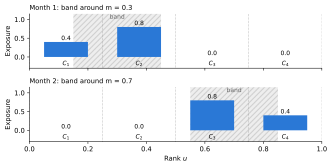
The second-moment matrix of the sorts is then
(\Psi_P)_{kl} = P^2 \int_{C_k} \int_{C_l} K(u, v)\, du\, dv, \qquad K(u, v) = \operatorname{E}_m[\beta(u, m)\, \beta(v, m)] = (2\ell - |u - v|)^+,
away from the edges of [0, 1]. K(u, v) is the probability that the band covers both ranks. As the groups get finer, \lambda_j(\Psi_P) / P converges to the j-th eigenvalue of K, viewed as an operator on functions of the rank (Chernov et al. 2026, Appendix OA.F). That operator has infinitely many positive eigenvalues, so every eigenvalue of the sorts grows in proportion to P. If the band never moved, K(u, v) = \beta(u, m)\beta(v, m) would have a single positive eigenvalue and the sorts would have a cliff too: the movement of the state is what creates the directions.
grid = 2048
u = (np.arange(grid) + 0.5) / grid
sigma2 = 4.0
sizes, sorts = [250, 1000, 4000], [16, 64, 256]
rng = np.random.default_rng(0)

def band_kernel(ell):
    B = (np.abs(u[:, None] - u[None, :]) < ell) * 1.0   # beta(u, m) on the grid
    return B @ B.T / grid, B

def sort_spectrum(K, P):
    # (1/P) Psi_P: the kernel averaged over pairs of groups, divided by P
    Kb = K.reshape(P, grid // P, P, grid // P).mean(axis=(1, 3))
    return np.linalg.eigvalsh(Kb / P)[::-1]

sort_spec, stock_spec = {}, {}
for ell in (0.25, 0.05):
    K, B = band_kernel(ell)
    sort_spec[ell] = {P: sort_spectrum(K, P) for P in sorts}
    if ell == 0.25:
        c, c0 = (B.mean(axis=0) ** 2).mean(), (B ** 2).mean()
        stock_spec = {N: np.r_[(N - 1) * c + c0 + sigma2, np.full(N - 1, c0 - c + sigma2)] / N for N in sizes}
Figure 2 compares the spectra. Each eigenvalue is divided by the number of assets, N for stocks and P for sorts. An eigenvalue that grows in proportion to the number of assets then stays put as assets are added, while a bounded one falls.
colors = ["#d4a017", "#2a78d6", "#7a4fb5"]

fig, axes = plt.subplots(1, 3, figsize=(9, 3.4))
panels = [("Stocks", stock_spec, "N"), ("Sorts, $\\ell = 0.25$", sort_spec[0.25], "P"),
          ("Sorts, $\\ell = 0.05$", sort_spec[0.05], "P")]
for ax, (title, spec, n) in zip(axes, panels):
    for size, col, mk in zip(spec, colors, ["o", "s", "^"]):
        r = min(len(spec[size]), 256)
        ax.plot(np.arange(1, r + 1), spec[size][:r], color=col, marker=mk, ms=2.5, linewidth=1, label=f"{n} = {size}")
    ax.set_xscale("log")
    ax.set_yscale("log")
    ax.set_title(title, fontsize=10)
    ax.set_xlabel("Rank $j$")
    ax.spines[["top", "right"]].set_visible(False)
    ax.legend(frameon=False, fontsize=8)
axes[0].set_ylabel("Eigenvalue / number of assets")
plt.tight_layout()
plt.show()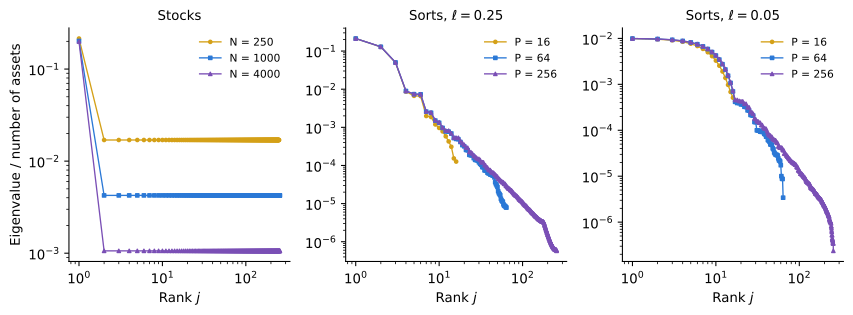
The stocks have a cliff: the first eigenvalue grows with N, and the rest fall in proportion to 1/N. The sorts have none. The curves for 16, 64 and 256 groups lie on top of each other, so every eigenvalue grows in proportion to P, and a finer sort adds eigenvalues further down. Only the last few eigenvalues of each coarse sort bend down, because coarse groups cannot resolve the finest directions.
The width of the band sets the shape. With a wide band, three eigenvalues stand out and the rest decline steadily. A finite-factor reading would see a cliff after three factors, yet every eigenvalue after the third grows like P as well. With a narrow band, about ten eigenvalues are nearly equal before the decline starts: the narrower the band, the more independent groups of stocks the factor can hit, and the more directions of risk the sorts span. Menus other than sorts, such as the random nonlinear weights of Didisheim et al. (2023), show a different shape in the model of Chernov et al. (2026, Theorem 4).
Didisheim, Antoine, Shikun Barry Ke, Bryan T. Kelly, and Semyon Malamud. 2023. Complexity in Factor Pricing Models. Working Paper No. 31689. National Bureau of Economic Research.
The spectrum of the factor zoo
The 153 factors of Jensen et al. (2023) are sorts too, but a different menu from the one above. Each month, each factor sorts stocks into thirds on one characteristic, with breakpoints from that month’s cross-section. Instead of finer and finer groups on one characteristic, the menu adds new characteristics, each sorted coarsely. The model shows why sorts can span many directions; with these factors the question is how many they span, not why.
Jensen, Theis Ingerslev, Bryan Kelly, and Lasse Heje Pedersen. 2023. “Is There a Replication Crisis in Finance?” The Journal of Finance 78 (5): 2465–518.
We use the full sample of 650 months, November 1971 to December 2025, and the second-moment matrix as in the previous notebook. The first component accounts for 51% of the trace and the first five for 80%, the usual pattern of a few dominant factors.
X = F.to_numpy()
T_all, N_all = X.shape

def eig2(Y):
    return np.linalg.eigvalsh(Y.T @ Y / len(Y))[::-1]

def shuffle(E):
    return np.column_stack([rng.permutation(E[:, i]) for i in range(E.shape[1])])

lam_full, V_full = np.linalg.eigh(X.T @ X / T_all)
lam_full, V_full = lam_full[::-1], V_full[:, ::-1]

pd.Series((lam_full / lam_full.sum())[:10].cumsum(), index=range(1, 11),
name="Cumulative share of trace").round(2).to_frame().T| 1 | 2 | 3 | 4 | 5 | 6 | 7 | 8 | 9 | 10 | |
|---|---|---|---|---|---|---|---|---|---|---|
| Cumulative share of trace | 0.51 | 0.66 | 0.73 | 0.77 | 0.8 | 0.83 | 0.84 | 0.86 | 0.87 | 0.88 |
Whether the rest is a bounded bulk is a question about how eigenvalues grow, which a single matrix cannot answer. We draw random subsets of P = 40 and 80 factors, 50 of each size, compute the eigenvalues of each, divide them by P, and compare them with those of all 153, as in Figure 2. Sampling noise also creates eigenvalues, and to see what it alone produces we repeat the exercise with each factor’s returns shuffled in time independently of the others. Shuffling keeps each factor’s mean and variance and destroys all comovement.
subsets = [40, 80, 153]
draws = {P: [rng.choice(N_all, P, replace=False) for _ in range(1 if P == N_all else 50)] for P in subsets}

def subset_spectrum(Y, P, nmax=40):
    return np.mean([eig2(Y[:, c])[:nmax] for c in draws[P]], axis=0) / P

X_shuf = shuffle(X)
spec_data = {P: subset_spectrum(X, P) for P in subsets}
spec_shuf = {P: subset_spectrum(X_shuf, P) for P in subsets}
fig, ax = plt.subplots(figsize=(8, 4.5))
r = np.arange(1, 41)
for P, col, mk in zip(subsets, colors, ["o", "s", "^"]):
ax.plot(r, spec_data[P], color=col, marker=mk, ms=3.5, label=f"Factors, P = {P}")
ax.plot(r, spec_shuf[P], color=col, marker=mk, ms=3.5, mfc="white", linestyle="--", label=f"Shuffled, P = {P}")
ax.set_xscale("log")
ax.set_yscale("log")
ax.xaxis.set_major_formatter(StrMethodFormatter("{x:g}"))
ax.set_xlabel("Rank $j$")
ax.set_ylabel("Eigenvalue / $P$")
ax.grid(axis="y", color="#e5e5e5", linewidth=0.8)
ax.spines[["top", "right"]].set_visible(False)
ax.legend(frameon=False, ncol=2)
plt.tight_layout()
plt.show()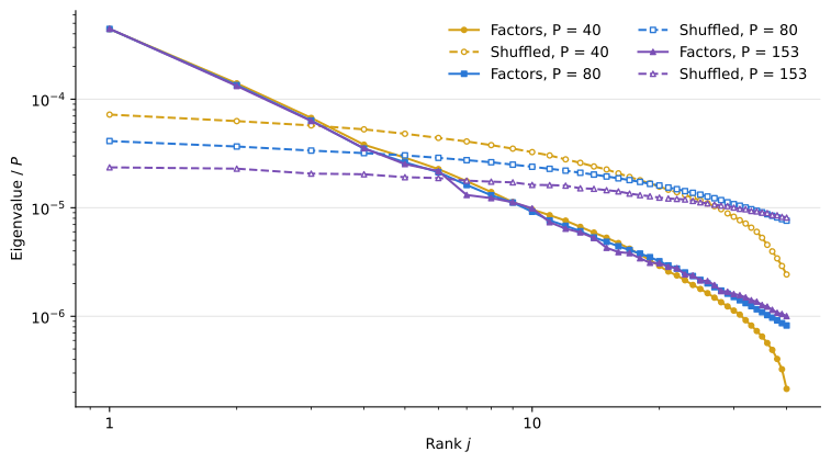
Up to about rank 20, the eigenvalues of the factors grow in proportion to P: the three solid curves coincide. The shuffled eigenvalues fall as P grows, as a bounded bulk should, although by less than 1/P, because the factors’ variances differ. Beyond rank 6 the factors’ eigenvalues lie below the shuffled ones: comovement concentrates the total variance in the leading components and leaves less for the rest. What separates them from noise is how they grow, not their size.
The shuffled factors have no comovement at all, which makes them an easy benchmark to beat. The relevant alternative is a cliff after K factors. To build one, we keep the projection of the factors on their first K full-sample components and shuffle the remainder in time, which leaves exactly K common directions plus noise with the factors’ own residual variances. Figure 4 repeats the subset exercise for K = 5, 15 and 30 and summarizes each spectrum by one number per rank: the eigenvalue over P with 40 factors divided by the same with all 153. Growth in proportion to P gives a ratio of one. A bounded eigenvalue gives a ratio above one, up to 153/40 \approx 3.8.
def null_k(K):
    common = X @ V_full[:, :K] @ V_full[:, :K].T
    return common + shuffle(X - common)

growth = {"Factors": spec_data[40] / spec_data[153], "Shuffled": spec_shuf[40] / spec_shuf[153]}
for K in (5, 15, 30):
    Y = null_k(K)
    growth[f"{K}-factor null"] = subset_spectrum(Y, 40) / subset_spectrum(Y, 153)
growth = pd.DataFrame(growth, index=range(1, 41))
fig, ax = plt.subplots(figsize=(8, 4.5))
styles = {"Factors": ("#222222", "-", "o"), "Shuffled": ("#888888", "--", "x"),
"5-factor null": ("#eb6834", "--", "s"), "15-factor null": ("#2a78d6", "--", "^"),
"30-factor null": ("#3a9e5c", "--", "D")}
rr = growth.index[:25]
for name, (col, ls, mk) in styles.items():
ax.plot(rr, growth.loc[rr, name], color=col, linestyle=ls, marker=mk, ms=4, label=name)
ax.axhline(1, color="#bbbbbb", linewidth=0.8)
ax.set_xlabel("Rank $j$")
ax.set_ylabel("Ratio, 40 factors to 153")
ax.grid(axis="y", color="#e5e5e5", linewidth=0.8)
ax.spines[["top", "right"]].set_visible(False)
ax.legend(frameon=False)
plt.tight_layout()
plt.show()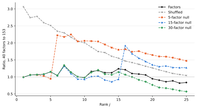
A cliff after 5 factors would have been obvious: the ratio of the 5-factor null jumps above 2 at rank 6, while that of the factors stays near one. A cliff after 15 factors shows up just as clearly at rank 16. A model with 30 common directions tracks the data up to about rank 20. So the factors span at least 20 or so pervasive directions of risk, far more than the 3 to 6 of the usual factor models. With 153 factors from a single sample, the data cannot say whether the number is 30 or infinite, a limit Chernov et al. (2026) note about this kind of evidence. Past rank 20 the ratios of the factors and of the 30-factor null drift below one, an artifact of approaching the last eigenvalues of the 40-factor subsets, so the comparison is informative only up to about rank 20.
Which components are priced?
Large eigenvalues are about risk. Whether a component earns a premium is a separate question, and the SDF needs only the components that do. In sample, every component looks priced, because each has some nonzero sample mean. Out of sample, Kozak et al. (2018) find that components beyond the first few add nothing.
Chernov, Mikhail, Bryan T. Kelly, Semyon Malamud, and Johannes Schwab. 2026. Infinite Factor Structure in Conditional Asset Pricing. Working Paper No. 35910. National Bureau of Economic Research.
We repeat their exercise with rolling windows, which they report gives the same results as their split sample. Each month we compute the components of the second-moment matrix of the past T months, with eigenvalues \lambda_j, eigenvectors v_j and component means m_j = v_j^\top \bar F. In the spirit of the groups of Chernov et al. (2026), which collect components whose eigenvalues grow at the same rate, we group the components by rank and form the SDF of each group, the portfolio \sum_{j} (m_j / \lambda_j)\, v_j over the components in the group. This is the ridgeless SDF of the previous notebook restricted to the group. We record its return in the next month, after scaling it to a gross exposure of one. All Sharpe ratios are annualized. With a window of 120 months there are only 120 components, so the last group holds components 81 to 120.
groups = [(1, 1), (2, 5), (6, 10), (11, 20), (21, 40), (41, 80), (81, 153)]
Ks = [1, 2, 3, 5, 8, 10, 15, 20, 25, 30, 40, 50, 75, 100, 153]
zs = np.r_[0.0, 10.0 ** np.arange(-4, 1.01, 0.5)]
z_best, rp_weight = zs[8], 10

def unit(w):
    return w / np.abs(w).sum()

def pc_portfolios(W):
    T, N = W.shape
    mu = W.mean(axis=0)
    _, s, Vt = np.linalg.svd(W / np.sqrt(T), full_matrices=False)
    lam, m = s ** 2, Vt @ mu
    port = {}
    for lo, hi in groups:
        port["group", f"{lo}+" if hi == N else f"{lo}-{hi}" if hi > lo else f"{lo}"] = \
            unit(Vt[lo - 1:hi].T @ (m[lo - 1:hi] / lam[lo - 1:hi]))
    for K in Ks:
        port["PCA", K] = unit(Vt[:K].T @ (m[:K] / lam[:K]))
    # Risk-premium PCA: components of the second-moment matrix plus a weight on the means
    _, U = np.linalg.eigh(W.T @ W / T + rp_weight * np.outer(mu, mu))
    U = U[:, ::-1]
    for K in Ks:
        Fk = W @ U[:, :K]
        # Minimum-norm solution: with T < N the matrix is singular for large K
        wf = np.linalg.lstsq(Fk.T @ Fk / T, Fk.mean(axis=0), rcond=1e-10)[0]
        port["RP-PCA", K] = unit(U[:, :K] @ wf)
    scale = lam.sum() / N
    for z in zs[1:]:
        a = z * scale
        port["Ridge", z] = unit(Vt.T @ (m / (lam + a)) + (mu - Vt.T @ m) / a)
    return port

def rolling(F, T, start="1992-01"):
    X, idx = F.to_numpy(), F.index
    t0 = idx.get_loc(pd.Period(start, "M"))
    rows = []
    for t in range(t0, len(idx)):
        port = pc_portfolios(X[t - T:t])
        rows.append([w @ X[t] for w in port.values()])
    return pd.DataFrame(rows, index=idx[t0:], columns=pd.MultiIndex.from_tuples(port.keys()))

windows = [120, 240]
R = {T: rolling(F, T) for T in windows}
sr = pd.DataFrame({T: sharpe(R[T]) for T in windows})
gsr = sr.loc["group"]
x = np.arange(len(gsr))
fig, ax = plt.subplots(figsize=(8, 4))
for i, (T, col) in enumerate(zip(windows, ["#2a78d6", "#3a9e5c"])):
ax.bar(x + (i - 0.5) * 0.38, gsr[T], width=0.38, color=col, hatch=["", "//"][i], edgecolor="white", label=f"T = {T}")
ax.axhline(0, color="#888888", linewidth=0.8)
ax.set_xticks(x, gsr.index)
ax.set_xlabel("Component ranks")
ax.set_ylabel("Sharpe ratio")
ax.grid(axis="y", color="#e5e5e5", linewidth=0.8)
ax.spines[["top", "right"]].set_visible(False)
ax.legend(frameon=False)
plt.tight_layout()
plt.show()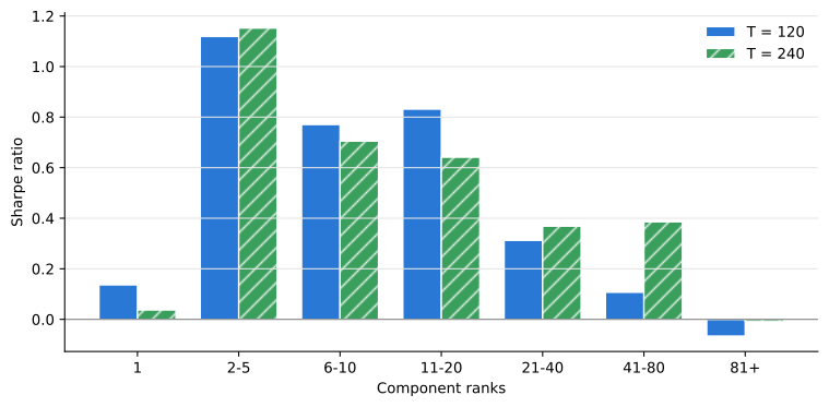
Over 408 months, the standard error of a Sharpe ratio near one is about 0.2, so differences of 0.1 or 0.2 between bars are noise. The first component earns little, about 0.1. Components 2 to 5 have a Sharpe ratio above one, and components 6 to 10 and 11 to 20 earn 0.6 to 0.85, clearly above zero and about the Sharpe ratio of the market. From rank 21 on the premia fade, to 0.1 to 0.4 for ranks 21 to 80, which a standard error of 0.2 mostly cannot distinguish from zero, and to nothing for the last group. The deepest components may carry no premium, or one too small to estimate with a window of 10 or 20 years, since their sample variance is tiny and their weights m_j / \lambda_j amplify the noise in m_j.
The first component is not the average factor, although its return has a correlation of 0.92 with the average. Its weights tilt toward the low-risk factors, which buy stocks with low volatility and sell those with high volatility, and Table 1 shows what that does.
pc1 = pd.Series(X @ V_full[:, 0], index=F.index)
pc1 *= np.sign(pc1.mean())
avg = F.mean(axis=1)

def describe(r):
    beta = np.cov(r, mkt)[0, 1] / mkt.var()
    return pd.Series({"Correlation with market": np.corrcoef(r, mkt)[0, 1], "Market beta": beta,
                      "Sharpe ratio": sharpe(r), "Sharpe ratio, market hedged": sharpe(r - beta * mkt)})

pd.DataFrame({"First component": describe(pc1), "Average factor": describe(avg)}).T.round(2)| Correlation with market | Market beta | Sharpe ratio | Sharpe ratio, market hedged | |
|---|---|---|---|---|
| First component | -0.50 | -2.83 | 0.23 | 0.54 |
| Average factor | -0.55 | -0.12 | 0.78 | 1.27 |
The low-risk factors are short the market, and the first component inherits a market beta of about -2.8. The equity premium it gives up offsets most of its anomaly premium. Hedged against the market, it earns 0.54. The market itself is not one of the 153 factors, so the SDF here prices the factors among themselves and is close to market neutral, as the previous notebook found.
Truncation out of sample
The groups are now combined. The PCA SDF keeps the first K components, the ridgeless SDF restricted to them. Lettau and Pelger (2020) argue that PCA picks components by variance alone and misses weak factors with high Sharpe ratios. Their risk-premium PCA (RP-PCA) instead takes the components of \frac{1}{T} \sum_s F_s F_s^\top + 10\, \bar F \bar F^\top, which tilts them toward directions with large means, and we form the tangency portfolio of the first K of them. Both are compared with the ridge SDF of the previous notebook at its best penalty, z = 0.32, which keeps every component and shrinks each one. Here, as in the previous notebook, components come from the second-moment matrix rather than the covariance matrix used by Kozak et al. (2018).
fig, ax = plt.subplots(figsize=(8, 4.5))
for T, col in zip(windows, ["#2a78d6", "#3a9e5c"]):
    ax.plot(Ks, sr.loc["PCA", T].to_numpy(), color=col, marker="o", ms=4, label=f"PCA, T = {T}")
    ax.plot(Ks, sr.loc["RP-PCA", T].to_numpy(), color=col, marker="s", ms=4, linestyle="--", label=f"RP-PCA, T = {T}")
    ax.axhline(sr.loc[("Ridge", z_best), T], color=col, linestyle=":", linewidth=1.2, label=f"Ridge, T = {T}")
ax.set_xscale("log")
ax.xaxis.set_major_formatter(StrMethodFormatter("{x:g}"))
ax.set_xlabel("Number of components $K$")
ax.set_ylabel("Sharpe ratio")
ax.grid(axis="y", color="#e5e5e5", linewidth=0.8)
ax.spines[["top", "right"]].set_visible(False)
ax.legend(frameon=False, ncol=3, fontsize=9)
plt.tight_layout()
plt.show()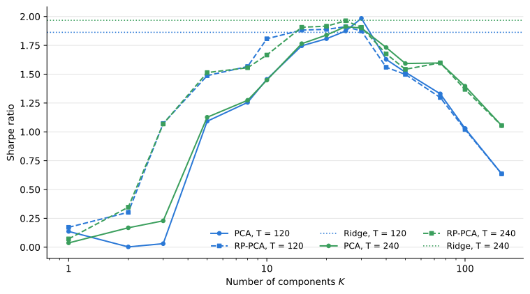
tbl = pd.concat({"PCA": sr.loc["PCA"], "RP-PCA": sr.loc["RP-PCA"]}, axis=1)
tbl.loc["Ridge, all"] = [sr.loc[("Ridge", z_best), T] for T in windows] * 2
tbl.index.name = "K"
tbl.round(2)| PCA | RP-PCA | |||
|---|---|---|---|---|
| 120 | 240 | 120 | 240 | |
| K | ||||
| 1 | 0.14 | 0.04 | 0.17 | 0.07 |
| 2 | 0.00 | 0.17 | 0.30 | 0.35 |
| 3 | 0.03 | 0.23 | 1.07 | 1.07 |
| 5 | 1.09 | 1.13 | 1.49 | 1.51 |
| 8 | 1.26 | 1.27 | 1.57 | 1.56 |
| 10 | 1.46 | 1.45 | 1.81 | 1.67 |
| 15 | 1.75 | 1.76 | 1.88 | 1.91 |
| 20 | 1.81 | 1.84 | 1.89 | 1.92 |
| 25 | 1.87 | 1.91 | 1.91 | 1.96 |
| 30 | 1.98 | 1.90 | 1.87 | 1.91 |
| 40 | 1.63 | 1.73 | 1.56 | 1.68 |
| 50 | 1.52 | 1.59 | 1.50 | 1.54 |
| 75 | 1.33 | 1.60 | 1.30 | 1.60 |
| 100 | 1.03 | 1.40 | 1.02 | 1.37 |
| 153 | 0.64 | 1.05 | 0.64 | 1.05 |
| Ridge, all | 1.86 | 1.97 | 1.86 | 1.97 |
Five components are not enough. With either window, the PCA SDF of 5 components has a Sharpe ratio of about 1.1, against 1.9 to 2.0 for the ridge SDF. RP-PCA helps where Lettau and Pelger (2020) say it should, among the leading components. With 3 components it reaches a Sharpe ratio of 1.07, where PCA earns almost nothing, and from 5 to 10 components it stays ahead by 0.2 to 0.4, because the weight on means moves high-premium directions forward. Between 15 and 30 components the two methods are within about 0.15 of each other. The Sharpe ratio keeps rising until 20 to 30 components, where both reach the ridge SDF, and then falls as the ridgeless weights on the deepest components bring in noise.
Lettau, Martin, and Markus Pelger. 2020. “Factors That Fit the Time Series and Cross-Section of Stock Returns.” Review of Financial Studies 33 (5): 2274–325.
Both the best K and the best penalty z = 0.32 are known only after the fact. A fair comparison chooses both in real time. Each month, as in the previous notebook, we pick the K of the PCA SDF and the z of the ridge SDF with the highest Sharpe ratio on past out-of-sample returns, after a burn-in of 60 months, so the comparison starts in January 1997.
def select(R, burn=60):
    # Each month, the column with the highest Sharpe ratio on past out-of-sample returns
    s = (R.expanding(burn).mean() / R.expanding(burn).std()).shift(1).dropna(how="all")
    best = s.idxmax(axis=1)
    return pd.Series([R.at[t, k] for t, k in best.items()], index=best.index), best

def se_diff(a, b):
    # Standard error of the difference of two annualized Sharpe ratios, i.i.d. returns
    n, s1, s2 = len(a), a.mean() / a.std(), b.mean() / b.std()
    c = np.corrcoef(a, b)[0, 1]
    return np.sqrt(12 * (2 - 2 * c + 0.5 * (s1 ** 2 + s2 ** 2 - 2 * s1 * s2 * c ** 2)) / n)

realtime, rt_rows = {}, {}
for T in windows:
    pca_rt, k_best = select(R[T]["PCA"])
    ridge_rt, _ = select(R[T]["Ridge"])
    realtime[T] = {"PCA, real-time K": pca_rt, "Ridge, real-time z": ridge_rt,
                   "PCA, K = 5": R[T]["PCA"][5].loc[pca_rt.index],
                   "Ridge, z = 0.32": R[T]["Ridge"][z_best].loc[pca_rt.index]}
    col = {k: f"{sharpe(v):.2f}" for k, v in realtime[T].items()}
    col["Difference, real-time PCA minus ridge"] = f"{sharpe(pca_rt) - sharpe(ridge_rt):.2f}"
    col["Standard error of the difference"] = f"{se_diff(pca_rt, ridge_rt):.2f}"
    col["Most frequent K"] = ", ".join(str(k) for k in k_best.value_counts().index[:2])
    rt_rows[f"T = {T}"] = col
pd.DataFrame(rt_rows)| T = 120 | T = 240 | |
|---|---|---|
| PCA, real-time K | 1.74 | 1.61 |
| Ridge, real-time z | 1.61 | 1.67 |
| PCA, K = 5 | 1.04 | 0.99 |
| Ridge, z = 0.32 | 1.71 | 1.76 |
| Difference, real-time PCA minus ridge | 0.13 | -0.06 |
| Standard error of the difference | 0.11 | 0.10 |
| Most frequent K | 30, 20 | 25, 30 |
Chosen in real time, the two methods tie. The PCA SDF settles on 20 to 30 components and earns within 0.15 of the ridge SDF, a difference of about one standard error or less. Truncation and shrinkage are both ways to regularize the estimate, as Kozak et al. (2018) point out, and with this menu both arrive at the same place: an SDF with 20 to 30 effective components, about five times as many as the usual factor models.
The gap at five components is also uneven over time. The previous notebook found that the SDF earned most of its Sharpe ratio before 2005, and Table 4 splits the sample at the same date.
periods = {"1992-2004": ("1992-01", "2004-12"), "2005-2025": ("2005-01", "2025-12")}
cols = {}
for T in windows:
    S = {"PCA, K = 5": R[T]["PCA"][5], "PCA, K = 25": R[T]["PCA"][25], "Ridge, z = 0.32": R[T]["Ridge"][z_best],
         **{f"Components {g}": R[T]["group"][g] for g in ["2-5", "6-10", "11-20", "21-40"]}}
    for p, (a, b) in periods.items():
        col = {k: f"{sharpe(v.loc[a:b]):.2f}" for k, v in S.items()}
        x5, xr = S["PCA, K = 5"].loc[a:b], S["Ridge, z = 0.32"].loc[a:b]
        col["K = 5 minus ridge"] = f"{sharpe(x5) - sharpe(xr):.2f}"
        col["Standard error"] = f"{se_diff(x5, xr):.2f}"
        cols[f"T = {T}", p] = col
pd.DataFrame(cols)| T = 120 | T = 240 | |||
|---|---|---|---|---|
| 1992-2004 | 2005-2025 | 1992-2004 | 2005-2025 | |
| PCA, K = 5 | 1.50 | 0.80 | 1.38 | 0.95 |
| PCA, K = 25 | 3.07 | 1.21 | 3.27 | 1.10 |
| Ridge, z = 0.32 | 2.93 | 1.19 | 3.23 | 1.21 |
| Components 2-5 | 1.50 | 0.85 | 1.40 | 0.98 |
| Components 6-10 | 1.43 | 0.32 | 1.44 | 0.19 |
| Components 11-20 | 1.12 | 0.65 | 0.86 | 0.48 |
| Components 21-40 | 0.19 | 0.39 | 0.59 | 0.21 |
| K = 5 minus ridge | -1.43 | -0.39 | -1.85 | -0.27 |
| Standard error | 0.34 | 0.24 | 0.36 | 0.23 |
From 1992 to 2004 the ridge SDF has a Sharpe ratio near 3, and the 5-component SDF falls short by 1.4 to 1.9, more than four standard errors. From 2005 to 2025 every SDF earns less, and the gap shrinks to 0.3 to 0.4, about one to one and a half standard errors. Components 2 to 5 and 11 to 20 still earn about 0.5 to 1.0 after 2005, while components 6 to 10 earn little. The case against five components is strong over the whole sample and in the early years, and suggestive since.
What we learned
The 153 factors have no cliff after the first few components. Random subsets show at least 20 or so directions whose eigenvalues grow with the number of factors, and a factor model with 5 or 15 common directions would have looked different. Whether the number is finite cannot be settled with one menu of 153 factors. In the band model, sorts lose the cliff because which stocks load on a factor changes from month to month. The data are consistent with this but cannot isolate it: many characteristics with many weak common factors would fit as well.
Components well beyond the first few are priced out of sample. Components 2 to 20 earn Sharpe ratios of 0.6 to 1.1 over 1992 to 2025, and an SDF needs 20 to 30 components to match the ridge SDF that keeps them all, whether K and z are chosen after the fact or in real time. Truncating to 5 gives up almost half of the Sharpe ratio over the full sample, mostly before 2005. Kozak et al. (2018) found 3 components enough among 15 anomalies, and expected a richer menu to need more; with ten times as many characteristics it needs several times as many components.
Kozak, Serhiy, Stefan Nagel, and Shrihari Santosh. 2018. “Interpreting Factor Models.” Journal of Finance 73 (3): 1183–223.
Ross, Stephen A. 1976. “The Arbitrage Theory of Capital Asset Pricing.” Journal of Economic Theory 13 (3): 341–60.
The near-arbitrage argument needs both a bound on Sharpe ratios and a cliff. The bound is the harder part to pin down. The Sharpe ratios near 2 here are on paper, before trading costs, which matter for factors that trade small stocks and rebalance often, and they come from a set of factors chosen after their publication. By the bound Ross (1976) suggests, a squared Sharpe ratio of at most twice the market’s, a Sharpe ratio of 2 would count as a near-arbitrage, and the sharp decline after 2005 is what one would expect if arbitrageurs competed part of it away. What the data do show is that wherever the bound sits, the premia are spread over many components, so a model with a handful of factors cannot capture them.
The factor menu here is narrow, one tertile sort per characteristic. The theory predicts more directions still for menus whose weights respond to the state, such as factors scaled by functions of past information. That is the subject of a later notebook.