import io
import re
import urllib.request
import zipfile
import numpy as np
import pandas as pd
import matplotlib.pyplot as plt
from _portfolio import DATA_DIR, load_wrds, load_wrds_by_year, summarize, sharpe

stocks = load_wrds("jkp_usa_stocks_1963_2025", """
    SELECT id, permno, eom AS date, me, crsp_exchcd, size_grp, prc,
           ret_exc, ret_exc_lead1m, dolvol_126d, bidaskhl_21d,
           be_me, ope_be, ret_12_1, ret_1_0, at_gr1
    FROM contrib_global_factor.global_factor
    WHERE excntry = 'USA' AND common = 1 AND exch_main = 1
      AND primary_sec = 1 AND obs_main = 1
      AND eom BETWEEN '1963-01-01' AND '2025-12-31'
""")

daily = load_wrds_by_year("crsp_dsf_1963_2025", """
    SELECT permno, dlycaldt AS date, dlyret AS ret, dlyprc AS prc,
           shrout, dlyvol AS vol, dlycap AS cap, siccd, primaryexch
    FROM crsp.dsf_v2
    WHERE dlycaldt BETWEEN '{year}-01-01' AND '{year}-12-31'
      AND sharetype = 'NS' AND securitytype = 'EQTY'
      AND securitysubtype = 'COM' AND usincflg = 'Y'
      AND issuertype IN ('ACOR', 'CORP')
      AND primaryexch IN ('N', 'A', 'Q')
      AND conditionaltype IN ('RW', 'NW')
""", range(1963, 2026))

# Daily effective spreads from the WRDS Intraday Indicators, averaged by month
year_sql = """
    SELECT l.permno, date_trunc('month', i.date)::date AS date,
           avg(i.effectivespread_percent_dw) AS espread
    FROM taqmsec.wrds_iid_{y} i
    JOIN wrdsapps_link_crsp_taqm.taqmclink l
      ON l.date = i.date AND l.sym_root = i.sym_root
     AND coalesce(l.sym_suffix, '') = coalesce(i.sym_suffix, '')
    WHERE i.effectivespread_percent_dw > 0
    GROUP BY 1, 2"""
taq = load_wrds("taq_effective_spreads_2003_2024",
                " UNION ALL ".join(year_sql.format(y=y) for y in range(2003, 2025)))

FRENCH = "https://mba.tuck.dartmouth.edu/pages/faculty/ken.french/ftp/"

def french_text(file):
    path = DATA_DIR / f"french_{file.removesuffix('.zip')}.txt"
    if not path.exists():
        z = zipfile.ZipFile(io.BytesIO(urllib.request.urlopen(FRENCH + file).read()))
        path.write_bytes(z.read(z.namelist()[0]))
    return path.read_text(encoding="latin1")

def french(file, table=0):
    """Table `table` of a file from Ken French's library, in decimals,
    indexed by day or by month."""
    blocks, rows, header = [], None, ""
    for line in french_text(file).splitlines():
        if re.fullmatch(r"\d{6}|\d{8}", line.split(",")[0].strip()):
            if rows is None:
                rows = [header]
                blocks.append(rows)
            rows.append(line)
        else:
            rows, header = None, line
    df = pd.read_csv(io.StringIO("\n".join(blocks[table])), index_col=0)
    df.columns = df.columns.str.strip()
    idx = df.index.astype(str).str.strip()
    df.index = (pd.to_datetime(idx, format="%Y%m%d") if len(idx[0]) == 8
                else pd.to_datetime(idx, format="%Y%m").to_period("M"))
    return df.astype(float).where(lambda x: x > -99) / 100

ff_d = french("F-F_Research_Data_Factors_daily_CSV.zip")
ff_m = french("F-F_Research_Data_Factors_CSV.zip")
umd_d = french("F-F_Momentum_Factor_daily_CSV.zip").iloc[:, 0]
umd_m = french("F-F_Momentum_Factor_CSV.zip").iloc[:, 0]
intl = pd.DataFrame({name: french(f).iloc[:, 0] for name, f in (
    ("Developed", "Developed_Mom_Factor_CSV.zip"),
    ("Developed ex US", "Developed_ex_US_Mom_Factor_CSV.zip"),
    ("Emerging", "Emerging_MOM_Factor_CSV.zip"))})
mom10 = french("10_Portfolios_Prior_12_2_CSV.zip")
ind30 = french("30_Industry_Portfolios_daily_CSV.zip")
rf, mex = ff_m["RF"], ff_m["Mkt-RF"]
Momentum Crashes
Momentum, buying the stocks that rose most over the past year and selling those that fell most, has earned high average returns in U.S. stocks since Jegadeesh and Titman (1993) and in most markets and asset classes since (Asness et al. 2013). It has also had the worst crashes of the common factors. In its Fall 2026 outlook, BlackRock’s systematic equity group reports that a global momentum strategy had its third-worst drawdown since 2000 from March through August 2026, a reversal of what had become consensus positioning, and says that it now monitors crowding alongside its signals (BlackRock 2026).
Jegadeesh, Narasimhan, and Sheridan Titman. 1993. “Returns to Buying Winners and Selling Losers: Implications for Stock Market Efficiency.” Journal of Finance 48 (1): 65–91.
Asness, Clifford S., Tobias J. Moskowitz, and Lasse Heje Pedersen. 2013. “Value and Momentum Everywhere.” Journal of Finance 68 (3): 929–85.
BlackRock. 2026. Hedge Fund Outlook, Fall 2026. BlackRock, for professional and institutional investors.
Three papers turn these remarks into something an investor can measure. Daniel and Moskowitz (2016) show that crashes are partly predictable: they come after market declines, when volatility is high, and at the moment the market rebounds, because the stocks that fell most behave like call options on the market. Barroso and Santa-Clara (2015) show that scaling momentum by its own recent volatility avoids most crashes and nearly doubles its Sharpe ratio. Lou and Polk (2022) measure crowding from returns alone: when the past winners and losers move together more than common factors explain, many arbitrageurs hold the same positions, and momentum’s returns over the following two years are lower.
This notebook rebuilds momentum from stock data, looks at its crashes, tests whether volatility scaling and the dynamic strategy of Daniel and Moskowitz (2016) survive in our sample and net of trading costs, and asks whether comomentum still predicts momentum’s returns in the decade after the sample of Lou and Polk (2022) ended.
Data
The monthly characteristics come from Jensen et al. (2023), as in What Do Anomalies Cost to Trade?: U.S. common stocks on their primary listing from January 1963 to December 2025, with market capitalization, the return from twelve months to one month ago, price, the NYSE flag, and the spreads used in that notebook. Daily returns come from the CRSP daily stock file for the same years, common stocks of U.S. companies listed on the NYSE, AMEX or NASDAQ. We use CRSP’s current format, in which the daily return on a stock’s last trading day includes its delisting return, which matters for momentum because losers delist more often. The legacy format on WRDS ends in December 2024.
Jensen, Theis Ingerslev, Bryan Kelly, and Lasse Heje Pedersen. 2023. “Is There a Replication Crisis in Finance?” The Journal of Finance 78 (5): 2465–518.
The market, the risk-free rate, the Fama-French factors, the 30 industry portfolios and the momentum factors of the United States, developed markets and emerging markets come from Ken French’s data library, which runs through September 2026 and lets us look at the episode BlackRock describes.
Momentum and its crashes
At the end of each month, stocks are sorted into deciles by their return from twelve months to one month ago, skipping the last month to avoid short-term reversal. As in Daniel and Moskowitz (2016), the breakpoints use all stocks and each decile is value weighted, with membership fixed through the following month. We compute the deciles’ daily returns, weighting each stock by its market capitalization on the previous day, and compound them into monthly returns. The momentum strategy, WML, is long the winner decile and short the loser decile.
s = stocks.dropna(subset=["permno", "me", "ret_12_1"]).copy()
s = s.astype({"permno": int, "me": float, "ret_12_1": float, "prc": float, "crsp_exchcd": float,
              "ret_exc_lead1m": float, "bidaskhl_21d": float})
s["month"] = s["date"].dt.to_period("M")
s["dec"] = s.groupby("month")["ret_12_1"].transform(lambda x: pd.qcut(x, 10, labels=False)) + 1

d = daily[["permno", "date", "ret", "cap"]].astype({"permno": int, "ret": float, "cap": float})
d = d.sort_values(["permno", "date"])
d["w"] = d.groupby("permno")["cap"].shift()
d["month"] = d["date"].dt.to_period("M")
d = d.merge(s[["permno", "month", "dec"]].assign(month=s["month"] + 1), on=["permno", "month"])
d = d.dropna(subset=["ret", "w"])
d["rw"] = d["ret"] * d["w"]
g = d.groupby(["date", "dec"])
dec_d = (g["rw"].sum() / g["w"].sum()).unstack()
dec_m = (1 + dec_d).groupby(dec_d.index.to_period("M")).prod() - 1
wml_d = dec_d[10] - dec_d[1]
wml = dec_m[10] - dec_m[1]
months = wml.index
Table 1 shows the familiar pattern. Average returns rise from the losers to the winners, and WML earns 22% a year with a volatility of 30%, a Sharpe ratio of 0.73, the same as the 0.71 that Daniel and Moskowitz (2016) report for 1927 to 2013. Its returns are strongly negatively skewed. The WML of French’s library, which uses NYSE breakpoints, has a correlation of 0.92 with ours and a lower average return, since NYSE breakpoints put fewer small stocks in the extreme deciles.
excess = dec_m.sub(rf.loc[months], axis=0)
tbl = pd.DataFrame({"Mean (%)": 1200 * dec_m.mean(), "Volatility (%)": 100 * np.sqrt(12) * dec_m.std(),
                    "Sharpe ratio": np.sqrt(12) * excess.mean() / excess.std(), "Skewness": dec_m.skew()})
tbl.loc["WML"] = [1200 * wml.mean(), 100 * np.sqrt(12) * wml.std(), sharpe(wml), wml.skew()]
tbl.round(2)| Mean (%) | Volatility (%) | Sharpe ratio | Skewness | |
|---|---|---|---|---|
| dec | ||||
| 1 | -2.98 | 34.57 | -0.21 | 0.66 |
| 2 | 6.00 | 26.87 | 0.06 | 0.28 |
| 3 | 7.05 | 22.13 | 0.12 | 0.08 |
| 4 | 10.21 | 18.71 | 0.31 | 0.01 |
| 5 | 11.08 | 16.86 | 0.40 | -0.38 |
| 6 | 10.44 | 15.77 | 0.38 | -0.38 |
| 7 | 12.45 | 15.42 | 0.52 | -0.32 |
| 8 | 13.17 | 15.90 | 0.55 | -0.35 |
| 9 | 13.76 | 17.50 | 0.54 | -0.48 |
| 10 | 19.30 | 23.09 | 0.65 | -0.19 |
| WML | 22.28 | 30.43 | 0.73 | -1.15 |
french_wml = mom10.iloc[:, -1] - mom10.iloc[:, 0]
print(f"Correlation with French's decile WML: {wml.corr(french_wml.loc[months]):.2f}, "
      f"average return {1200 * french_wml.loc[months].mean():.1f}% a year")
Correlation with French's decile WML: 0.92, average return 13.8% a yearThe crashes are concentrated in a few months. The ten worst months of WML in Table 2 lost between 25% and 47%, and all ten came after 1990. Seven of them came when the market had fallen over the previous two years, and in all ten the market rose that month. In January 2001, after the technology stocks had become the losers, they rebounded and WML lost 47%. In March and April 2009 the financial stocks that had fallen most rebounded first, and WML lost 43% and 45%.
mkt = mex + rf
mret24 = (1 + mkt).rolling(24).apply(np.prod, raw=True) - 1
worst = wml.nsmallest(10).index
pd.DataFrame({"WML": 100 * wml.loc[worst], "Losers": 100 * dec_m.loc[worst, 1],
              "Winners": 100 * dec_m.loc[worst, 10], "Market": 100 * mkt.loc[worst],
"Market, past 24 months": 100 * mret24.shift(1).loc[worst]}).round(1)| WML | Losers | Winners | Market | Market, past 24 months | |
|---|---|---|---|---|---|
| date | |||||
| 2001-01 | -47.5 | 40.9 | -6.6 | 3.8 | 10.7 |
| 2009-04 | -45.1 | 44.4 | -0.6 | 10.2 | -40.5 |
| 2009-03 | -42.9 | 48.6 | 5.7 | 9.0 | -44.8 |
| 2002-11 | -37.5 | 40.7 | 3.2 | 6.1 | -36.1 |
| 2023-01 | -35.7 | 36.0 | 0.4 | 7.0 | -0.8 |
| 2020-04 | -32.7 | 48.3 | 15.6 | 13.6 | -0.7 |
| 2009-08 | -30.1 | 30.4 | 0.3 | 3.3 | -27.2 |
| 2001-11 | -26.4 | 31.1 | 4.7 | 7.7 | -19.6 |
| 2020-11 | -25.0 | 37.6 | 12.5 | 12.5 | 27.1 |
| 1991-02 | -24.8 | 34.2 | 9.4 | 7.7 | 19.5 |
The 2026 episode
BlackRock’s measure is a global momentum strategy. French’s library has momentum factors for developed markets, with and without the United States, and for emerging markets, built from sorts on size and past returns like UMD, the U.S. factor that averages large and small stocks. Table 3 shows them through September 2026, with the two U.S. series. In every region the main loss came in July, between 10% and 17%, after strong gains in April. In the United States the losses continued in August: French’s decile WML lost 22.7% in July and 14.4% in August, 33.9% over the two months, and UMD lost 17.1%. From March through August as a whole, no factor lost more than 3.4%, while their worst six months since 2000, all in 2009, cost between 35% and 80%. None of French’s factors, U.S. or international, shows the six-month drawdown BlackRock reports. Its strategy is its own, and the note to its chart does not say how it is weighted or scaled.
mom = pd.concat([umd_m.rename("UMD"), french_wml.rename("Decile WML"), intl], axis=1)
six = ((1 + mom).rolling(6).apply(np.prod, raw=True) - 1).loc["2000":]
tbl = 100 * mom.loc["2026-01":].T
tbl.columns = tbl.columns.strftime("%b")
tbl["Mar to Aug"] = 100 * six.loc["2026-08"]
tbl["Worst six months"] = 100 * six.min()
tbl.round(1)| Jan | Feb | Mar | Apr | May | Jun | Jul | Aug | Sep | Mar to Aug | Worst six months | |
|---|---|---|---|---|---|---|---|---|---|---|---|
| UMD | 5.0 | 1.3 | 1.6 | 9.5 | 1.4 | 4.6 | -12.2 | -5.6 | 6.7 | -2.2 | -54.2 |
| Decile WML | 6.3 | 2.0 | -1.0 | 25.2 | 16.7 | 15.4 | -22.7 | -14.4 | 16.7 | 10.4 | -80.0 |
| Developed | 4.6 | 2.6 | -0.8 | 10.3 | 2.1 | 2.6 | -11.9 | -2.3 | 5.6 | -1.4 | -42.3 |
| Developed ex US | 6.8 | 4.6 | -2.6 | 6.9 | 1.5 | 0.4 | -10.1 | 1.4 | 5.3 | -3.4 | -40.2 |
| Emerging | 8.0 | 5.5 | -5.0 | 12.8 | 9.6 | 0.4 | -16.8 | 8.0 | 5.9 | 5.9 | -35.3 |
Table 4 ranks the two-month loss against all others since 2000, counting each episode once. For the decile WML it is the second worst, behind spring 2009; for UMD it is the fifth worst. The U.S. data agree with BlackRock that 2026 brought one of the sharpest momentum reversals of the century, though over two months rather than six.
def worst_windows(r, k=2, n=6):
    c = ((1 + r).rolling(k).apply(np.prod, raw=True) - 1).loc["2000":]
    out = []
    while len(out) < n:
        t = c.idxmin()
        out.append((str(t), round(100 * c[t], 1)))
        c = c[(c.index < t - (k - 1)) | (c.index > t + (k - 1))]
    return out

pd.concat({name: pd.DataFrame(worst_windows(r), columns=["Ending", "Return"])
for name, r in (("Decile WML", french_wml), ("UMD", umd_m))}, axis=1)| Decile WML | UMD | |||
|---|---|---|---|---|
| Ending | Return | Ending | Return | |
| 0 | 2009-04 | -66.7 | 2009-05 | -42.6 |
| 1 | 2026-08 | -33.9 | 2002-11 | -21.0 |
| 2 | 2002-11 | -33.2 | 2001-01 | -20.4 |
| 3 | 2021-03 | -33.2 | 2003-05 | -19.0 |
| 4 | 2001-02 | -33.1 | 2026-08 | -17.1 |
| 5 | 2023-02 | -32.1 | 2000-05 | -16.8 |
When momentum crashes
Daniel and Moskowitz (2016) explain why the crashes come in rebounds. After a bear market the loser decile is full of stocks that fell with the market, often firms close to distress whose equity behaves like a call option on the firm. When the market turns up, these stocks rise more than their betas imply, and a portfolio short the losers is short a call. They measure this with the regression R^e_{i,t} = (\alpha_0 + \alpha_B I_{B,t-1}) + \left[\beta_0 + I_{B,t-1}(\beta_B + I_{U,t} \, \beta_{B,U})\right] R^e_{m,t} + \varepsilon_t, \tag{1} where I_{B,t-1} is one if the market’s return over the previous 24 months is negative, I_{U,t} is one if the market’s excess return R^e_{m,t} is positive this month, and \beta_{B,U} is the extra beta in up markets after a bear market.
def ols(y, X):
    Xc = np.column_stack([np.ones(len(y)), X])
    b = np.linalg.lstsq(Xc, y, rcond=None)[0]
    e = y - Xc @ b
    se = np.sqrt(np.diag(np.linalg.inv(Xc.T @ Xc)) * (e @ e) / (len(y) - Xc.shape[1]))
    return b, b / se

bear = (mret24 < 0).astype(float).shift(1).loc[months]
up = (mex > 0).astype(float).loc[months]
m_ex = mex.loc[months]
Z = np.column_stack([bear, m_ex, bear * m_ex, bear * up * m_ex])
names = ["alpha_0", "alpha_B", "beta_0", "beta_B", "beta_BU"]
rows = {}
for name, y in (("Losers", dec_m[1] - rf.loc[months]), ("Winners", dec_m[10] - rf.loc[months]), ("WML", wml)):
    b, t = ols(y.to_numpy(), Z)
    b[:2] *= 100
    rows[name] = pd.Series(np.ravel(np.column_stack([b, t])),
                           index=pd.MultiIndex.from_product([names, ["coef", "t"]]))
pd.DataFrame(rows).T.round(2)| alpha_0 | alpha_B | beta_0 | beta_B | beta_BU | ||||||
|---|---|---|---|---|---|---|---|---|---|---|
| coef | t | coef | t | coef | t | coef | t | coef | t | |
| Losers | -1.86 | -7.23 | 0.50 | 0.40 | 1.50 | 24.13 | 0.29 | 1.21 | 0.63 | 1.67 |
| Winners | 0.56 | 3.68 | -0.57 | -0.78 | 1.31 | 35.43 | -0.41 | -2.95 | 0.05 | 0.23 |
| WML | 2.42 | 7.46 | -1.07 | -0.69 | -0.19 | -2.43 | -0.70 | -2.35 | -0.58 | -1.21 |
The pattern is there, though weaker than in their longer sample. In bear markets the losers’ beta in up markets rises by 0.63 and the winners’ by almost nothing, so WML’s falls by 0.58. The t-statistic on WML’s coefficient is only -1.2: our sample starts in 1963 and misses the 1930s, the decade with the largest rebounds, which drive their estimate. The effect on average returns is clearer. In column (1) of Table 6 below, WML earns 2.3% a month outside bear markets and loses 1.2% a month after one.
The second result of Daniel and Moskowitz (2016) is that the crashes can be forecast with information available in advance. Their Table 5 regresses WML on the bear market indicator, the variance of daily market returns over the previous 126 days, \hat\sigma^2_{m,t-1}, and their product. We scale the variance by its average over bear markets, \bar v_B, so that the interaction has an average of one when I_B = 1.
mvar = ff_d["Mkt-RF"].rolling(126).var()
mvar = mvar.groupby(mvar.index.to_period("M")).last().shift(1)
vB = mvar.loc[months][bear == 1].mean()
X = pd.DataFrame({"I_B": bear, "Variance": mvar.loc[months] / vB, "I_B x variance": bear * mvar.loc[months] / vB})
specs = [["I_B"], ["Variance"], ["I_B", "Variance"], ["I_B x variance"], ["I_B", "Variance", "I_B x variance"]]
out = {}
for i, spec in enumerate(specs, 1):
    b, t = ols(wml.to_numpy(), X[spec].to_numpy())
    out[f"({i})"] = pd.Series({k: f"{100 * bk:.2f} ({tk:.1f})" for k, bk, tk in zip(["Intercept"] + spec, b, t)})
pd.DataFrame(out).reindex(["Intercept", "I_B", "Variance", "I_B x variance"]).fillna("")| (1) | (2) | (3) | (4) | (5) | |
|---|---|---|---|---|---|
| Intercept | 2.32 (6.8) | 2.91 (7.4) | 2.99 (7.6) | 2.37 (7.4) | 2.16 (4.9) |
| I_B | -3.55 (-3.8) | -2.30 (-2.3) | 0.96 (0.8) | ||
| Variance | -2.41 (-4.4) | -1.91 (-3.3) | 0.45 (0.6) | ||
| I_B x variance | -3.99 (-6.5) | -4.79 (-4.1) |
Both forecast low returns. The interaction alone has a t-statistic of -6.5: after a bear market with average variance, WML’s expected return falls by about 4 percentage points a month, which more than offsets the intercept of 2.4%. With all three variables, the interaction takes the effect, as in Daniel and Moskowitz (2016).
Managing the risk
If momentum’s crashes come when its volatility is high, an investor can scale the position down when volatility rises. Barroso and Santa-Clara (2015) estimate the variance of WML each month from its daily returns over the previous 126 trading days, \hat\sigma^2_{t} = 21 \sum_{j=0}^{125} \frac{r^2_{\text{WML},d_t - j}}{126}, and hold w_t = \sigma_{\text{target}} / \hat\sigma_t of WML in month t + 1, with an annualized target of 12%. The strategy remains self-financing; only the size of the long and short positions changes.
Daniel and Moskowitz (2016) go one step further. Maximizing the unconditional Sharpe ratio gives a weight proportional to the conditional Sharpe ratio divided by the volatility, w_t = \frac{1}{2\lambda} \frac{\mu_t}{\sigma^2_t}, so volatility scaling is optimal only if the Sharpe ratio of WML is constant. It is not, since the mean falls after bear markets with high variance. Their dynamic strategy forecasts \mu_t with the fitted interaction regression of Table 6, column (4), and \sigma^2_t with a GJR-GARCH model combined with realized volatility. We use the realized variance alone for \sigma^2_t, and estimate the mean regression each month with data up to that month only, which is their out-of-sample version. The first 120 months are used to start the regression, so the comparison runs from January 1974.
rv = (wml_d ** 2).rolling(126).mean() * 21
rv = rv.groupby(rv.index.to_period("M")).last().shift(1)
w_cvol = 0.12 / np.sqrt(12 * rv)

inter = (bear * mvar).reindex(months)
mu = pd.Series(np.nan, index=months)
for i in range(120, len(months)):
    past = months[:i]
    b, _ = ols(wml.loc[past].to_numpy(), inter.loc[past].to_numpy())
    mu.iloc[i] = b[0] + b[1] * inter.iloc[i]
w_dyn = mu / rv.loc[months]

oos = pd.period_range("1974-01", "2025-12", freq="M")
managed = pd.DataFrame({"WML": wml, "Constant volatility": w_cvol * wml, "Dynamic": w_dyn * wml}).loc[oos]
# Scale each strategy after the fact to the volatility of WML, which leaves Sharpe ratios unchanged
vol = managed["WML"].std()
scale = vol / managed.std()
managed = managed * scale
tbl = {}
for c in managed:
st = summarize(managed[c] + rf.loc[oos], mkt.loc[oos], rf.loc[oos])
st["Skewness"] = managed[c].skew()
st["Excess kurtosis"] = managed[c].kurt()
st["Worst month (%)"] = 100 * managed[c].min()
tbl[c] = st
pd.DataFrame(tbl).round(2)| WML | Constant volatility | Dynamic | |
|---|---|---|---|
| Mean (%) | 25.09 | 36.72 | 39.14 |
| Volatility (%) | 32.00 | 32.05 | 32.08 |
| Sharpe ratio | 0.65 | 1.02 | 1.09 |
| Beta | -0.46 | -0.25 | 0.02 |
| Alpha (%) | 24.60 | 34.48 | 34.67 |
| Alpha p-value | 0.00 | 0.00 | 0.00 |
| Max drawdown (%) | -83.41 | -53.60 | -54.26 |
| Skewness | -1.14 | -0.23 | 1.30 |
| Excess kurtosis | 4.68 | 1.45 | 9.72 |
| Worst month (%) | -47.49 | -30.51 | -43.82 |
fig, ax = plt.subplots(figsize=(8, 4.5))
for c, col in zip(managed, ("#555555", "#2a78d6", "#d6452a")):
    ax.plot(managed.index.to_timestamp(), np.log1p(managed[c]).cumsum(), color=col, linewidth=1.6, label=c)
ax.set_xlabel("Year")
ax.set_ylabel("Cumulative log return")
ax.grid(axis="y", color="#e5e5e5", linewidth=0.8)
ax.spines[["top", "right"]].set_visible(False)
ax.legend(frameon=False)
plt.tight_layout()
plt.show()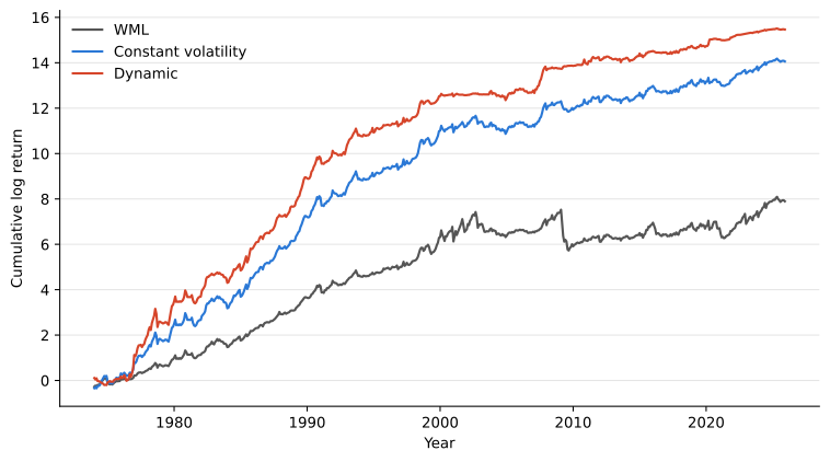
Scaling by volatility raises the Sharpe ratio of WML from 0.65 to 1.02 and cuts the maximum drawdown from 83% to 54%, at the same volatility. Skewness goes from -1.14 to -0.23. These are the results of Barroso and Santa-Clara (2015), who report a Sharpe ratio of 0.97 against 0.53 from 1927 to 2011. The weight in WML averages 0.65 and falls to 0.15 in April 2009, when WML lost 45% and constant-volatility WML 13%.
The dynamic strategy reaches 1.09, a little more than constant volatility, with positive skewness. It also shows the risk Daniel and Moskowitz (2016) warn about: its weight varies far more, between -1.5 and 7.7 times WML after scaling, and its worst month, a loss of 44% in October 1978, came in a calm period in which the low forecast variance made the position several times larger than WML. Table 8 shows that both managed strategies beat WML in each half of the sample. Since 2000, when momentum crashed most, they earn Sharpe ratios of 0.58 and 0.72 against 0.37.
periods = {"1974-1999": ("1974-01", "1999-12"), "2000-2025": ("2000-01", "2025-12"),
           "2016-2025": ("2016-01", "2025-12"), "1974-2025": ("1974-01", "2025-12")}
pd.DataFrame({p: managed.loc[a:b].apply(sharpe) for p, (a, b) in periods.items()}).round(2)| 1974-1999 | 2000-2025 | 2016-2025 | 1974-2025 | |
|---|---|---|---|---|
| WML | 1.18 | 0.37 | 0.48 | 0.65 |
| Constant volatility | 1.39 | 0.58 | 0.60 | 1.02 |
| Dynamic | 1.40 | 0.72 | 0.82 | 1.09 |
The same rule applied to UMD with French’s daily data shows how it behaved in 2026. After the gains of the spring, the trailing volatility of UMD had risen, and the weight fell from 0.79 in March to 0.57 in July and 0.50 in August. The scaled factor lost 6.9% and 2.8% in those months, against 12.2% and 5.6% for UMD.
rv_u = (umd_d ** 2).rolling(126).mean() * 21
w_u = 0.12 / np.sqrt(12 * rv_u.groupby(rv_u.index.to_period("M")).last().shift(1))
pd.DataFrame({"Weight": w_u, "UMD": 100 * umd_m, "Scaled UMD": 100 * w_u * umd_m}).loc["2026-01":].round(2).T| 2026-01 | 2026-02 | 2026-03 | 2026-04 | 2026-05 | 2026-06 | 2026-07 | 2026-08 | 2026-09 | |
|---|---|---|---|---|---|---|---|---|---|
| Weight | 0.78 | 0.83 | 0.79 | 0.70 | 0.68 | 0.65 | 0.57 | 0.50 | 0.50 |
| UMD | 5.03 | 1.31 | 1.56 | 9.51 | 1.39 | 4.62 | -12.21 | -5.60 | 6.70 |
| Scaled UMD | 3.94 | 1.09 | 1.24 | 6.66 | 0.94 | 2.98 | -6.92 | -2.79 | 3.37 |
Crowding
Lou and Polk (2022) measure how crowded momentum is from the returns of the stocks it holds. If many arbitrageurs buy the same winners and sell the same losers, their trades move these stocks together beyond what common factors explain. At the end of each month they take the stocks in the extreme deciles, compute weekly returns over the previous 52 weeks, subtract the return of each stock’s Fama-French industry and remove the three Fama-French factors with a regression over the same weeks. Comomentum is the average correlation of each stock’s residual with that of the rest of its decile, \text{CoMOM}^L = \frac{1}{N^L} \sum_{i=1}^{N^L} \text{Corr}\left(r^L_i, r^L_{-i} \mid \text{MKT}, \text{SMB}, \text{HML}\right), \qquad \text{CoMOM} = \tfrac{1}{2}\left(\text{CoMOM}^L + \text{CoMOM}^W\right), where r^L_{-i} is the equal-weighted return of the loser decile without stock i, and likewise for the winners. They exclude stocks below $5 and in the bottom NYSE size decile, and sort the remaining stocks into deciles. We require a stock to have all 52 weekly returns.
# Fama-French 30 industries from SIC codes
lut, ind = np.full(10000, 30), None
for line in french_text("Siccodes30.zip").splitlines():
    if m := re.match(r"^\s*(\d+)\s+[A-Za-z]", line):
        ind = int(m[1])
    elif m := re.match(r"^\s+(\d{4})-(\d{4})", line):
        lut[int(m[1]):int(m[2]) + 1] = ind

# Weekly (Friday to Friday) returns net of the stock's industry
dw = daily[["permno", "date", "ret", "siccd"]].dropna(subset=["ret"]).astype({"permno": int, "ret": float})
dw["ind"] = lut[dw["siccd"].fillna(9999).astype(int).clip(0, 9999).to_numpy()]
dw["week"] = dw["date"].dt.to_period("W-FRI")
dw["lr"] = np.log1p(dw["ret"])
g = dw.groupby(["permno", "week"])
wk = pd.DataFrame({"r": np.expm1(g["lr"].sum()), "ind": g["ind"].last()}).reset_index()
ind_w = np.expm1(np.log1p(ind30).groupby(ind30.index.to_period("W-FRI")).sum(min_count=1))
ind_w.columns = range(1, 31)
ind_w = ind_w.stack().rename("ir")
ind_w.index.names = ["week", "ind"]
wk = wk.join(ind_w, on=["week", "ind"])
R = (wk["r"] - wk["ir"]).groupby([wk["week"], wk["permno"]]).first().unstack()

# Weekly Fama-French factors
compound = lambda x: np.expm1(np.log1p(x).groupby(x.index.to_period("W-FRI")).sum())
ff_w = pd.DataFrame({"MKT": compound(ff_d["Mkt-RF"] + ff_d["RF"]) - compound(ff_d["RF"]),
                     "SMB": compound(ff_d["SMB"]), "HML": compound(ff_d["HML"])})

# Deciles in the universe of Lou and Polk
nyse10 = s[s["crsp_exchcd"] == 1].groupby("month")["me"].quantile(0.1)
lp = s[(s["prc"].abs() >= 5) & (s["me"] >= s["month"].map(nyse10))].copy()
lp["dec"] = lp.groupby("month")["ret_12_1"].transform(lambda x: pd.qcut(x, 10, labels=False)) + 1

Rv, cols = R.to_numpy(), {p: i for i, p in enumerate(R.columns)}
week_end = R.index.end_time.normalize()
Fv = ff_w.reindex(R.index).to_numpy()

def comom(members, rows):
    X = Rv[np.ix_(rows, [cols[p] for p in members if p in cols])]
    X = X[:, ~np.isnan(X).any(axis=0)]
    n = X.shape[1]
    F = np.column_stack([np.ones(len(rows)), Fv[rows]])
    E = X - F @ np.linalg.lstsq(F, X, rcond=None)[0]
    L = (E.sum(axis=1, keepdims=True) - E) / (n - 1)
    E, L = E - E.mean(axis=0), L - L.mean(axis=0)
    return ((E * L).sum(axis=0) / np.sqrt((E ** 2).sum(axis=0) * (L ** 2).sum(axis=0))).mean()

out = {}
for m, g in lp.groupby("month"):
    rows = np.where(week_end <= m.end_time.normalize())[0][-52:]
    if len(rows) < 52:
        continue
    mid = g.loc[g["dec"].isin([5, 6]), "permno"]
    out[m] = {"Losers": comom(g.loc[g["dec"] == 1, "permno"], rows),
              "Winners": comom(g.loc[g["dec"] == 10, "permno"], rows),
              "Deciles 5 and 6": comom(mid.sample(min(400, len(mid)), random_state=0), rows)}
C = pd.DataFrame(out).T
C["CoMOM"] = (C["Losers"] + C["Winners"]) / 2
The middle deciles are included as a control, from a random sample of 400 stocks each month to keep the computation short. Over 1965 to 2011, the main sample of Lou and Polk (2022), our comomentum averages 0.091, 0.097 for the losers and 0.085 for the winners (Table 10). They report 0.092, 0.098 and 0.086 in their Table 1. The middle deciles average 0.035, so the extreme deciles move together far more than the typical stock. Figure 2 shows that comomentum was high around 2000 and 2009, as they find, and that it has stayed high since 2015, averaging 0.130 since 2012 and reaching 0.21 in July 2025, its highest level since 2009. The middle deciles also moved together unusually in the second half of 2025, at 0.12 to 0.17, so part of that peak is comovement across all stocks rather than among momentum stocks alone.
fig, ax = plt.subplots(figsize=(8, 3.5))
ax.plot(C.index.to_timestamp(), C["CoMOM"], color="#2a78d6", linewidth=1.4, label="CoMOM")
ax.plot(C.index.to_timestamp(), C["Deciles 5 and 6"], color="#999999", linewidth=1.0, label="Deciles 5 and 6")
ax.set_xlabel("Year")
ax.set_ylabel("Average correlation")
ax.grid(axis="y", color="#e5e5e5", linewidth=0.8)
ax.spines[["top", "right"]].set_visible(False)
ax.legend(frameon=False)
plt.tight_layout()
plt.show()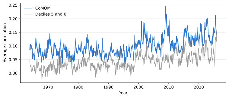
pd.DataFrame({p: C.loc[a:b].mean() for p, (a, b) in {"1965-2011": ("1965-01", "2011-12"), "2012-2025": ("2012-01", "2025-12")}.items()}).round(3)| 1965-2011 | 2012-2025 | |
|---|---|---|
| Losers | 0.097 | 0.152 |
| Winners | 0.085 | 0.108 |
| Deciles 5 and 6 | 0.035 | 0.069 |
| CoMOM | 0.091 | 0.130 |
The test of Lou and Polk (2022) is whether comomentum predicts momentum’s returns over the next two years. For each formation month, we hold the value-weighted winner and loser deciles of their universe, fixed at formation, for 24 months, and record the return of the winners minus the losers in the formation year (year 0), the first year after formation (year 1) and the second (year 2). As they do, we first remove from comomentum its relation to the market’s return and volatility over the previous 24 months, then sort the formation months into quintiles.
P = s[["permno", "month", "me", "ret_exc_lead1m"]].dropna()
ext = lp.loc[lp["dec"].isin([1, 10]), ["permno", "month", "dec", "me", "ret_12_1"]]
leg = lambda e, col: (e["me"] * e[col]).groupby([e["form"], e["dec"]]).sum() / e["me"].groupby([e["form"], e["dec"]]).sum()
y0 = leg(ext.rename(columns={"month": "form"}), "ret_12_1").unstack()
H = {}
for h in range(1, 25):
    e = ext[["permno", "month", "dec"]].assign(form=ext["month"], month=ext["month"] + (h - 1))
    r = leg(e.merge(P, on=["permno", "month"]), "ret_exc_lead1m").unstack()
    H[h] = r[10] - r[1]
H = pd.DataFrame(H)
event = pd.DataFrame({"Year 0": y0[10] - y0[1], "Year 1": H.loc[:, 1:12].sum(axis=1),
                      "Year 2": H.loc[:, 13:24].sum(axis=1)})

mvol24 = mkt.rolling(24).std()

def orthogonal(x):
    Z = np.column_stack([np.ones(len(x)), mret24.loc[x.index], mvol24.loc[x.index]])
    return x - Z @ np.linalg.lstsq(Z, x.to_numpy(), rcond=None)[0]

def quintiles(a, b):
    x = orthogonal(C["CoMOM"].loc[a:b])
    q = pd.qcut(x, 5, labels=False) + 1
    t = (100 * event.loc[x.index].groupby(q).mean()).T
    t["5 - 1"] = t[5] - t[1]
return tpd.concat({"1965-2011": quintiles("1965-01", "2011-12"), "2012-2023": quintiles("2012-01", "2023-12")}).round(1)| CoMOM | 1 | 2 | 3 | 4 | 5 | 5 - 1 | |
|---|---|---|---|---|---|---|---|
| 1965-2011 | Year 0 | 130.1 | 138.9 | 133.3 | 164.6 | 185.9 | 55.8 |
| Year 1 | 10.9 | 11.8 | 9.2 | 6.0 | -0.4 | -11.3 | |
| Year 2 | 1.4 | -4.2 | -5.8 | -7.0 | -8.5 | -9.9 | |
| 2012-2023 | Year 0 | 147.6 | 147.5 | 147.8 | 143.4 | 125.5 | -22.1 |
| Year 1 | 13.5 | 4.0 | 14.8 | 0.2 | -5.7 | -19.2 | |
| Year 2 | 5.3 | -1.7 | 2.2 | -1.7 | -3.5 | -8.8 |
The result of Lou and Polk (2022) holds in our data. From 1965 to 2011, momentum formed when comomentum is in its top quintile earns 11 percentage points less in the first year than when it is in the bottom quintile, and another 10 points less in the second year. They report 12.7 points over the first year and a further 13 points over the second. In the twelve years since their main sample, the difference is larger, 19 points in the first year and 9 in the second, although the formation-year return is not higher in the top quintile, as it is in their sample.
Newey, Whitney K., and Kenneth D. West. 1987. “A Simple, Positive Semi-Definite, Heteroskedasticity and Autocorrelation Consistent Covariance Matrix.” Econometrica 55 (3): 703–8.
The formation months overlap, so year-1 returns of neighboring months share eleven months of data. Table 12 regresses the returns on the percentile rank of comomentum with Newey and West (1987) standard errors, using 12 lags for year 1 and 24 for year 2. The slopes are negative in every period, but the t-statistics are between -0.9 and -1.9. With overlapping returns, 47 years contain fewer than 24 independent two-year observations, and the twelve years since then fewer than six.
def newey_west(y, x, lags):
    X = np.column_stack([np.ones(len(y)), x])
    b = np.linalg.lstsq(X, y, rcond=None)[0]
    u = X * (y - X @ b)[:, None]
    S = u.T @ u
    for l in range(1, lags + 1):
        G = u[l:].T @ u[:-l]
        S += (1 - l / (lags + 1)) * (G + G.T)
    Q = np.linalg.inv(X.T @ X)
    return b[1], b[1] / np.sqrt((Q @ S @ Q)[1, 1])

slopes = {}
for p, (a, b) in {"1965-2011": ("1965-01", "2011-12"), "2012-2023": ("2012-01", "2023-12")}.items():
    rank = orthogonal(C["CoMOM"].loc[a:b]).rank(pct=True)
    slopes[p] = {col: "{:.1f} ({:.1f})".format(*newey_west(100 * event.loc[rank.index, col].to_numpy(), rank.to_numpy(), L))
                 for col, L in (("Year 1", 12), ("Year 2", 24))}
pd.DataFrame(slopes)| 1965-2011 | 2012-2023 | |
|---|---|---|
| Year 1 | -13.8 (-1.9) | -20.7 (-1.5) |
| Year 2 | -10.5 (-1.3) | -10.2 (-0.9) |
Comomentum has also drifted up. Every month since 2015 is above the median of 1965 to 2014, so an investor ranking comomentum against its own past in real time would have been told for a decade that momentum was crowded. The quintiles above are formed within each period, with hindsight about the drift. In July 2025 comomentum reached its highest level since 2009, and twelve months later U.S. momentum had its sharpest reversal since then. That is one episode, consistent with the paper, not evidence for it.
Trading costs
Volatility scaling changes the size of the position every month, which adds trades, but it also holds less of WML on average, which removes them. To price both, we follow What Do Anomalies Cost to Trade?: the weights of each stock drift with returns over the month, the trade is the change to the new weights, and each dollar traded pays half the bid-ask spread, either the high-low estimate of Corwin and Schultz (2012) or the TAQ effective spread from 2004 to 2024. For constant-volatility WML the new position is w_t times the WML weights, and the drifted position is w_{t-1} times the drifted weights.
Corwin, Shane A., and Paul Schultz. 2012. “A Simple Way to Estimate Bid-Ask Spreads from Daily High and Low Prices.” Journal of Finance 67 (2): 719–60.
e = s.loc[s["dec"].isin([1, 10])].dropna(subset=["ret_exc_lead1m"]).copy()
taq_m = taq.astype({"permno": float, "espread": float}).assign(month=taq["date"].dt.to_period("M"))
e = e.merge(taq_m[["permno", "month", "espread"]].astype({"permno": int}), on=["permno", "month"], how="left")
e["side"] = np.where(e["dec"] == 10, 1.0, -1.0)
e["w"] = e["side"] * e["me"] / e.groupby(["month", "dec"])["me"].transform("sum")
e["leg_ret"] = (e["w"] * e["ret_exc_lead1m"]).groupby([e["month"], e["dec"]]).transform("sum") * e["side"]
e["drift"] = e["w"] * (1 + e["ret_exc_lead1m"]) / (1 + e["leg_ret"])
k = w_cvol.shift(-1)  # weight chosen at the end of month t for month t + 1
T = e[["id", "month", "w", "bidaskhl_21d", "espread"]].merge(
    e[["id", "month", "drift"]].assign(month=e["month"] + 1), on=["id", "month"], how="outer").fillna({"w": 0, "drift": 0})
T["bidaskhl_21d"] = T["bidaskhl_21d"].where(T["bidaskhl_21d"] > 0).fillna(T.groupby("month")["bidaskhl_21d"].transform("median"))
T["trade"] = (T["w"] - T["drift"]).abs()
T["trade_cvol"] = (T["month"].map(k) * T["w"] - T["month"].map(k.shift(1)) * T["drift"]).abs()

# Gross returns of the daily-based WML, indexed by the month of formation
gross = wml.shift(-1)
cost = pd.DataFrame({f"{c}, {spread}": (T[c] * T[col] / 2).groupby(T["month"]).sum(min_count=1)
                     for c in ("trade", "trade_cvol") for spread, col in (("high-low", "bidaskhl_21d"), ("TAQ", "espread"))})
res = pd.DataFrame({"WML": gross, "Constant volatility": gross * k})
cost_of = {"WML": "trade", "Constant volatility": "trade_cvol"}
def cost_table(idx, spreads):
rows = {}
for name, c in cost_of.items():
row = {"Turnover (%)": 100 * T[c].groupby(T["month"]).sum().loc[idx].mean() / 4,
"Gross (%)": 1200 * res[name].loc[idx].mean(), "Gross Sharpe": sharpe(res[name].loc[idx])}
for sp in spreads:
row[f"Cost, {sp} (%)"] = 1200 * cost[f"{c}, {sp}"].loc[idx].mean()
row[f"Net Sharpe, {sp}"] = sharpe((res[name] - cost[f"{c}, {sp}"]).loc[idx])
rows[name] = row
return pd.DataFrame(rows).T
# Formation months, so that returns run from January 1974 and January 2004
pd.concat({"1974-2025": cost_table(pd.period_range("1973-12", "2025-11", freq="M"), ["high-low"]),
"2004-2024": cost_table(pd.period_range("2003-12", "2024-11", freq="M"), ["high-low", "TAQ"])}).round(2).fillna("")| Turnover (%) | Gross (%) | Gross Sharpe | Cost, high-low (%) | Net Sharpe, high-low | Cost, TAQ (%) | Net Sharpe, TAQ | ||
|---|---|---|---|---|---|---|---|---|
| 1974-2025 | WML | 37.88 | 20.82 | 0.65 | 13.52 | 0.23 | ||
| Constant volatility | 25.49 | 16.21 | 1.02 | 8.80 | 0.47 | |||
| 2004-2024 | WML | 37.46 | 12.85 | 0.37 | 11.45 | 0.04 | 1.03 | 0.34 |
| Constant volatility | 19.81 | 8.56 | 0.65 | 5.52 | 0.23 | 0.54 | 0.61 |
WML replaces 38% of each leg a month, more than the 23% of the tercile momentum factor of the previous notebook, since decile portfolios are more extreme. Constant-volatility WML trades less, because its average weight is 0.65, and the monthly changes in the weight add less than the smaller positions save. With the high-low spreads, which overstate costs for large stocks, costs take most of WML’s return, and the Sharpe ratio net of costs is 0.23 against 0.47 for constant-volatility WML. With TAQ spreads after 2004, costs are about 1 percentage point a year for WML, and the net Sharpe ratios are 0.34 and 0.61. Volatility scaling survives trading costs.
What we learned
Momentum’s crashes are real and concentrated: its ten worst months since 1963 lost between a quarter and a half of the position, all after 1990, mostly in rebounds after bear markets. The 2026 reversal that BlackRock describes shows up in U.S. data as a two-month loss of 34% for the decile strategy in July and August, the second worst since 2000, and in French’s developed and emerging markets factors as a loss of 10% to 17% in July, rather than as a six-month drawdown.
Crashes are partly predictable, as Daniel and Moskowitz (2016) find. After a bear market with high volatility, the expected return of momentum is negative. Scaling momentum by its trailing volatility, as Barroso and Santa-Clara (2015) propose, raises its Sharpe ratio from 0.65 to 1.02 from 1974 to 2025, cuts the maximum drawdown from 83% to 54%, and removes most of the negative skewness. It also trades less than plain momentum, so the gain survives spreads. The dynamic strategy of Daniel and Moskowitz (2016) adds a little more, at the cost of much larger and more variable leverage.
Daniel, Kent, and Tobias J. Moskowitz. 2016. “Momentum Crashes.” Journal of Financial Economics 122 (2): 221–47.
Barroso, Pedro, and Pedro Santa-Clara. 2015. “Momentum Has Its Moments.” Journal of Financial Economics 116 (1): 111–20.
Lou, Dong, and Christopher Polk. 2022. “Comomentum: Inferring Arbitrage Activity from Return Correlations.” Review of Financial Studies 35 (7): 3272–302.
Crowding can be measured from returns. Our comomentum reproduces that of Lou and Polk (2022), and momentum formed when it is high earns less over the next two years, in their sample and in the twelve years after it. The statistical evidence is weak, since overlapping two-year returns give few independent observations, and comomentum has drifted up, so it does not give an investor a clear signal in real time. BlackRock’s advice to watch crowding alongside the signal is consistent with this evidence; acting on it mechanically would have meant holding little momentum for most of the past decade.