import numpy as np
import pandas as pd
import matplotlib.pyplot as plt
from _portfolio import load_wrds, load_jkp

stocks = load_wrds("jkp_usa_stocks_1963_2025", """
    SELECT id, permno, eom AS date, me, crsp_exchcd, size_grp, prc,
           ret_exc, ret_exc_lead1m, dolvol_126d, bidaskhl_21d,
           be_me, ope_be, ret_12_1, ret_1_0, at_gr1
    FROM contrib_global_factor.global_factor
    WHERE excntry = 'USA' AND common = 1 AND exch_main = 1
      AND primary_sec = 1 AND obs_main = 1
      AND eom BETWEEN '1963-01-01' AND '2025-12-31'
""")

# Daily effective spreads from the WRDS Intraday Indicators, averaged by month
year_sql = """
    SELECT l.permno, date_trunc('month', i.date)::date AS date,
           avg(i.effectivespread_percent_dw) AS espread
    FROM taqmsec.wrds_iid_{y} i
    JOIN wrdsapps_link_crsp_taqm.taqmclink l
      ON l.date = i.date AND l.sym_root = i.sym_root
     AND coalesce(l.sym_suffix, '') = coalesce(i.sym_suffix, '')
    WHERE i.effectivespread_percent_dw > 0
    GROUP BY 1, 2"""
taq = load_wrds("taq_effective_spreads_2003_2024",
                " UNION ALL ".join(year_sql.format(y=y) for y in range(2003, 2025)))

jkp = load_jkp("jkp_usa_all_factors_monthly_vw_cap",
               "https://jkpfactors-data.s3.amazonaws.com/public/"
               "%5Busa%5D_%5Ball_factors%5D_%5Bmonthly%5D_%5Bvw_cap%5D.zip")

num = stocks.columns.drop(["date", "size_grp"])
stocks[num] = stocks[num].astype(float)
stocks["month"] = stocks["date"].dt.to_period("M")
taq = taq.astype({"permno": float, "espread": float})
taq["month"] = taq["date"].dt.to_period("M")
stocks = stocks.merge(taq[["permno", "month", "espread"]], on=["permno", "month"], how="left")

J = jkp.assign(month=jkp["date"].dt.to_period("M")).pivot(index="month", columns="name", values="ret")
full = pd.period_range("1972-01", "2025-12", freq="M")
recent = pd.period_range("2004-01", "2024-12", freq="M")What Do Anomalies Cost to Trade?
The previous notebooks report gross returns. An investor who trades a factor pays a cost on every trade, and there is no agreement on how large that cost is. Three studies span the range.
Chen and Velikov (2023) estimate the expected return of 204 anomalies net of trading costs. The average anomaly earned 68 bps a month in its original sample before costs, 44 bps after costs, 9 bps after publication, and 4 bps after 2005. They charge half the effective bid-ask spread on every trade and leave out price impact, so these figures are an upper bound on what an investor nets.
Frazzini et al. (2018) measure costs directly, from $1.7 trillion of trades executed by a large institutional money manager in 21 developed markets from 1998 to 2016. The average market impact of those trades is about 10 bps, and they conclude that the costs assumed in academic studies are an order of magnitude too high, and the capacity of anomaly strategies an order of magnitude too low.
Novy-Marx and Velikov (2016) sit in between. Costs depend mostly on how much a strategy trades, and reduce its net return by more than 1% of its monthly one-sided turnover. Strategies that turn over less than half of their positions a month mostly survive costs once they are built to trade less, while few that turn over more do.
This notebook rebuilds six factors from stock-level data, measures how much they trade, and prices the trades three ways: with a spread estimated from daily prices, as in much of the academic literature, with effective spreads measured in intraday data, and with the market impact model of Frazzini et al. (2018).
Data
The factors of the previous notebooks come as returns, which say nothing about trades. To measure trades we need the stocks in each portfolio. Jensen et al. (2023) publish the characteristics behind their factors on WRDS, one row per stock and month, and we take the U.S. common stocks on their primary listing from January 1963 to December 2025: market capitalization, the characteristics of six factors, the excess return of the following month, average daily dollar volume over the past 126 trading days, and the bid-ask spread estimated from daily high and low prices over the past 21 days with the method of Corwin and Schultz (2012).
Corwin, Shane A., and Paul Schultz. 2012. “A Simple Way to Estimate Bid-Ask Spreads from Daily High and Low Prices.” Journal of Finance 67 (2): 719–60.
The second measure of spreads comes from TAQ, the record of every trade and quote on U.S. exchanges. The WRDS Intraday Indicators compute from it each stock’s daily effective spread, twice the distance between the trade price and the midpoint of the best quotes, as a percentage of the midpoint and weighted by dollar volume. We average it by month and link it to the stocks with the WRDS link table. Our subscription covers millisecond TAQ, which starts in September 2003, and the indicators run through December 2024.
Rebuilding the factors
The six factors are size, value (book-to-market), profitability (operating profits to book equity), investment (asset growth), momentum (the return from twelve months to one month ago) and short-term reversal (last month’s return). They are built as Jensen et al. (2023) build theirs. At the end of each month, stocks are sorted into terciles by the characteristic with breakpoints from NYSE stocks, and the factor is long the top tercile and short the bottom one, in the direction of the original study. Within each leg stocks are weighted by market capitalization capped at the 80th percentile of NYSE stocks, and each leg holds one dollar.
Jensen, Theis Ingerslev, Bryan Kelly, and Lasse Heje Pedersen. 2023. “Is There a Replication Crisis in Finance?” The Journal of Finance 78 (5): 2465–518.
Table 1 compares the rebuilt factors with the returns that Jensen et al. (2023) publish. The correlations are 0.96 or higher. Average returns differ by up to 0.7 percentage points a year, the most for value, which we have not traced. The comparisons below use the rebuilt factors throughout, gross and net, so these differences do not affect them.
# Name: (JKP factor, characteristic, sign of the long leg)
FACTORS = {
    "Size": ("market_equity", "me", -1),
    "Value": ("be_me", "be_me", 1),
    "Profitability": ("ope_be", "ope_be", 1),
    "Investment": ("at_gr1", "at_gr1", -1),
    "Momentum": ("ret_12_1", "ret_12_1", 1),
    "Short-term reversal": ("ret_1_0", "ret_1_0", -1),
}

def weights(stocks, char, sign, band=None):
    """Signed weights formed at each month end: long the top tercile of sign * char,
    short the bottom one, NYSE breakpoints, market caps capped at the NYSE 80th
    percentile. With band = (enter, exit), a stock enters a leg in the outer
    `enter` fraction and stays until it leaves the outer `exit` fraction."""
    d = stocks.dropna(subset=["me", char, "ret_exc_lead1m"])
    rows, longs, shorts = [], set(), set()
    for m, g in d.groupby("month"):
        s = sign * g[char]
        nyse = g["crsp_exchcd"] == 1
        q = s[nyse].quantile
        if band is None:
            L, S = s >= q(2 / 3), s <= q(1 / 3)
        else:
            enter, exit_ = band
            L = (s >= q(1 - enter)) | (g["id"].isin(longs) & (s >= q(1 - exit_)))
            S = (s <= q(enter)) | (g["id"].isin(shorts) & (s <= q(exit_)))
            longs, shorts = set(g.loc[L, "id"]), set(g.loc[S, "id"])
        w = g["me"].clip(upper=g.loc[nyse, "me"].quantile(0.8))
        w = pd.concat([w[L] / w[L].sum(), -w[S] / w[S].sum()])
        rows.append(pd.DataFrame({"month": m, "id": g.loc[w.index, "id"], "w": w.to_numpy()}))
    return pd.concat(rows, ignore_index=True)

def trades(W, stocks):
    """Gross return and trades of a long-short portfolio, both indexed by the
    month of the return. Trades are the change from the weights after a month
    of drift to the new weights."""
    W = W.merge(stocks[["id", "month", "ret_exc_lead1m"]], on=["id", "month"])
    W["leg"] = np.sign(W["w"])
    W["contrib"] = W["w"] * W["ret_exc_lead1m"]
    gross = W.groupby("month")["contrib"].sum()
    by_leg = W.groupby(["month", "leg"])
    W = W.join((by_leg["contrib"].sum() / by_leg["w"].sum()).rename("leg_ret"), on=["month", "leg"])
    W["drift"] = W["w"] * (1 + W["ret_exc_lead1m"]) / (1 + W["leg"] * W["leg_ret"])
    prev = W[["id", "month", "drift"]].assign(month=W["month"] + 1)
    T = W[["id", "month", "w"]].merge(prev, on=["id", "month"], how="outer").fillna({"w": 0, "drift": 0})
    T = T[T["month"].isin(W["month"].unique()[1:])]
    T["dw"] = (T["w"] - T["drift"]).abs()
    T = T.merge(stocks[["id", "month", "me", "bidaskhl_21d", "espread", "dolvol_126d"]],
                on=["id", "month"], how="left")
    for c in ("bidaskhl_21d", "dolvol_126d"):
        T[c] = T[c].where(T[c] > 0).fillna(T.groupby("month")[c].transform("median"))
    gross.index = gross.index + 1
    T["month"] = T["month"] + 1
    return gross, T

def turnover(T):
    # Share of each leg replaced per month, averaged over the two legs
    return T.groupby("month")["dw"].sum() / 4

def spread_cost(T, col):
    # Each dollar traded pays half the spread
    return (T["dw"] * T[col] / 2).groupby(T["month"]).sum(min_count=1)

port = {f: trades(weights(stocks, c, s), stocks) for f, (_, c, s) in FACTORS.items()}
gross = pd.DataFrame({f: port[f][0] for f in FACTORS})
pd.DataFrame({
"JKP factor": [FACTORS[f][0] for f in FACTORS],
"Correlation": [gross[f].loc[full].corr(J[FACTORS[f][0]].loc[full]) for f in FACTORS],
"Mean, rebuilt": [1200 * gross[f].loc[full].mean() for f in FACTORS],
"Mean, JKP": [1200 * J[FACTORS[f][0]].loc[full].mean() for f in FACTORS],
}, index=list(FACTORS)).round(2)| JKP factor | Correlation | Mean, rebuilt | Mean, JKP | |
|---|---|---|---|---|
| Size | market_equity | 1.00 | 0.22 | 0.25 |
| Value | be_me | 0.97 | 3.73 | 3.07 |
| Profitability | ope_be | 0.99 | 3.76 | 4.00 |
| Investment | at_gr1 | 0.96 | 3.35 | 3.75 |
| Momentum | ret_12_1 | 0.98 | 6.57 | 6.90 |
| Short-term reversal | ret_1_0 | 0.99 | 3.97 | 3.69 |
Turnover
Between rebalancing dates the weights drift with returns. The trade of stock i at the end of month t is the change from the drifted weight \tilde w_{i,t} to the new weight w_{i,t}, and turnover is the share of each leg replaced, \frac{1}{2} \sum_i |w_{i,t} - \tilde w_{i,t}|, averaged over the two legs. Paying a proportional cost c_{i,t} per dollar traded, the factor loses \text{Cost}_t = \sum_i |w_{i,t} - \tilde w_{i,t}| \, c_{i,t} \tag{1} in month t + 1, where the sum runs over both legs. With the bid-ask spread s_{i,t}, a trade at the bid or the ask pays half the spread, c_{i,t} = s_{i,t} / 2.
Table 2 shows that turnover depends on how fast the characteristic changes. Size and the accounting characteristics change slowly, and their factors replace 6% to 12% of each leg a month. Momentum replaces 23%, since the past year’s return changes each month by one month in and one out. Short-term reversal replaces 71%, almost all of the leg, since last month’s return is a new number every month.
turn = pd.DataFrame({f: turnover(port[f][1]) for f in FACTORS})
pd.DataFrame({"Turnover (%)": 100 * turn.loc[full].mean(),
"Gross return (%/yr)": 1200 * gross.loc[full].mean()}).round(2)| Turnover (%) | Gross return (%/yr) | |
|---|---|---|
| Size | 5.91 | 0.22 |
| Value | 9.76 | 3.73 |
| Profitability | 7.13 | 3.76 |
| Investment | 11.51 | 3.35 |
| Momentum | 23.26 | 6.57 |
| Short-term reversal | 70.85 | 3.97 |
Spreads
Table 3 compares the two spread measures where both exist. For the largest stocks the high-low estimate is 12 times the effective spread from TAQ, 52 bps against 4 bps. The ratio falls with size and is close to one only for the smallest stocks, the nano caps, whose spreads are about 2%.
both = stocks[stocks["month"].isin(recent)].dropna(subset=["espread", "bidaskhl_21d"])
order = ["mega", "large", "small", "micro", "nano"]
tbl = both.groupby("size_grp")[["espread", "bidaskhl_21d"]].median().loc[order] * 1e4
tbl.columns = ["TAQ effective", "High-low"]
tbl["Ratio"] = tbl["High-low"] / tbl["TAQ effective"]
tbl["Stock-months"] = both.groupby("size_grp").size().loc[order]
tbl.round(1)| TAQ effective | High-low | Ratio | Stock-months | |
|---|---|---|---|---|
| size_grp | ||||
| mega | 4.4 | 51.6 | 11.8 | 84693 |
| large | 7.3 | 62.8 | 8.6 | 154162 |
| small | 14.7 | 83.7 | 5.7 | 228238 |
| micro | 56.3 | 116.1 | 2.1 | 375381 |
| nano | 228.3 | 198.2 | 0.9 | 147783 |
Corwin, Shane A., and Paul Schultz. 2012. “A Simple Way to Estimate Bid-Ask Spreads from Daily High and Low Prices.” Journal of Finance 67 (2): 719–60.
def vw_spread(col):
    d = stocks.dropna(subset=[col, "me"])
    d = d[d[col] > 0]
    year = d["month"].dt.year
    return (d[col] * d["me"]).groupby(year).sum() / d["me"].groupby(year).sum()

hl_y = vw_spread("bidaskhl_21d").loc[1972:2025] * 1e4
taq_y = vw_spread("espread").loc[2004:2024] * 1e4
fig, ax = plt.subplots(figsize=(8, 3.5))
ax.plot(hl_y.index, hl_y, color="#2a78d6", linewidth=1.8, label="High-low estimate")
ax.plot(taq_y.index, taq_y, color="#d6452a", linewidth=1.8, label="TAQ effective spread")
ax.set_xlabel("Year")
ax.set_ylabel("Spread (basis points)")
ax.set_ylim(0, None)
ax.grid(axis="y", color="#e5e5e5", linewidth=0.8)
ax.spines[["top", "right"]].set_visible(False)
ax.legend(frameon=False)
plt.tight_layout()
plt.show()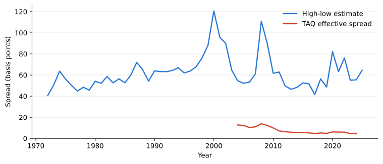
Returns net of spreads
Figure 1 shows the same gap over time. Value-weighted, the TAQ effective spread falls from 13 bps in 2004 to under 5 bps in 2024, while the high-low estimate stays between 40 and 65 bps in most years, with peaks of 121 bps in 2000, 111 bps in 2008 and 82 bps in 2020, years of high volatility. Chen and Velikov (2023) find the same upward bias of 25 to 50 bps after 2005 in all four estimators from daily data that they examine, the high-low estimate among them, and cite evidence that it is related to volatility. They use intraday spreads whenever they are available.
Table 4 applies 1 with each spread. With the high-low estimate, costs take 1.4 to 2.2 percentage points a year from the slow factors, 4.4 from momentum and 13.3 from short-term reversal. Over 1972 to 2025, size and short-term reversal lose money net of costs, and the other four keep between a third and two thirds of their gross return. The monthly cost is about 1.6% to 2% of monthly turnover, close to the rule of thumb of Novy-Marx and Velikov (2016).
From 2004 to 2024, TAQ spreads make costs about a seventh as large: 0.2 to 0.3 percentage points a year for the slow factors, 0.6 for momentum and 1.8 for short-term reversal. What changes the picture in this period is the gross return. Profitability still earns 3.6% a year, but value, investment, momentum and short-term reversal earn between 0.5% and 1.9%, and size loses money. Net of TAQ spreads, profitability keeps 3.4%, momentum 1.3% and investment 0.7%. With correct spreads, trading costs are small for factors that trade large stocks, and the decline of their gross returns matters more, which is the conclusion of Chen and Velikov (2023).
cost_hl = pd.DataFrame({f: spread_cost(port[f][1], "bidaskhl_21d") for f in FACTORS})
cost_taq = pd.DataFrame({f: spread_cost(port[f][1], "espread") for f in FACTORS})
pd.DataFrame({
    ("1972-2025", "Gross"): gross.loc[full].mean(),
    ("1972-2025", "Cost, high-low"): cost_hl.loc[full].mean(),
    ("1972-2025", "Net"): (gross - cost_hl).loc[full].mean(),
    ("2004-2024", "Gross"): gross.loc[recent].mean(),
    ("2004-2024", "Cost, high-low"): cost_hl.loc[recent].mean(),
    ("2004-2024", "Cost, TAQ"): cost_taq.loc[recent].mean(),
    ("2004-2024", "Net, TAQ"): (gross - cost_taq).loc[recent].mean(),
}).mul(1200).round(2)| 1972-2025 | 2004-2024 | ||||||
|---|---|---|---|---|---|---|---|
| Gross | Cost, high-low | Net | Gross | Cost, high-low | Cost, TAQ | Net, TAQ | |
| Size | 0.22 | 1.42 | -1.20 | -1.88 | 1.41 | 0.24 | -2.12 |
| Value | 3.73 | 1.96 | 1.77 | 0.50 | 1.73 | 0.25 | 0.25 |
| Profitability | 3.76 | 1.46 | 2.31 | 3.57 | 1.30 | 0.18 | 3.39 |
| Investment | 3.35 | 2.15 | 1.20 | 0.99 | 2.08 | 0.28 | 0.71 |
| Momentum | 6.57 | 4.41 | 2.16 | 1.85 | 4.25 | 0.58 | 1.27 |
| Short-term reversal | 3.97 | 13.32 | -9.34 | 0.65 | 12.80 | 1.81 | -1.15 |
Price impact and capacity
Spreads are the cost of a small trade. A larger trade moves the price, and the cost per dollar grows with the size of the trade relative to the stock’s volume. Frazzini et al. (2018) estimate the market impact of their trades, in basis points, as \text{MI}(x) = a + b \, x + c \sqrt{x}, where x is the trade as a percentage of the stock’s average daily dollar volume, and the intercept a holds the other variables of their model at their sample medians. We use the global estimates, b = -0.13 and c = 8.89 (Table VII, column 5), and read a, about 1 bp, from their Figure 6. The linear term is negative and not significant (t = -0.72), and if kept it makes the cost fall for trades above about 1,200% of daily volume, far beyond the trade sizes in their Figure 6, which stops at 12%. The authors themselves describe impact as a square root of trade size, so we drop the linear term and use \text{MI}(x) = 1 + 8.89 \sqrt{x}.
A fund with A dollars in each leg trades |w_{i,t} - \tilde w_{i,t}| A dollars of stock i, and pays \text{MI}(x_{i,t}) on each dollar in 1. We state A in dollars of December 2024 and scale it with the market capitalization of U.S. stocks, so that a fund of a given size holds the same share of the market in every year. We treat each month’s trade as executed in a single day, which overstates the impact of large trades that a fund would spread over several days.
# Market impact in basis points of a trade of x percent of daily dollar volume,
# Table VII, column (5) of Frazzini, Israel and Moskowitz, with the intercept
# read from their Figure 6 and without the linear term
def impact(x):
    return 1 + 8.89 * np.sqrt(x)

# Fund size per leg, in dollars of December 2024, scaled by the stock market
mkt = stocks.groupby("month")["me"].sum()
scale = mkt / mkt.loc[pd.Period("2024-12", "M")]

def impact_cost(T, aum):
    a = aum * scale.reindex(T["month"] - 1).to_numpy()
    x = 100 * T["dw"] * a / T["dolvol_126d"]
    return (T["dw"] * impact(x) / 1e4).groupby(T["month"]).sum()

sizes = 10.0 ** np.arange(7, 11.6, 0.25)
net_aum = {per: pd.DataFrame({f: [(gross[f] - impact_cost(port[f][1], A)).loc[idx].mean() * 1200
                                  for A in sizes] for f in FACTORS}, index=sizes)
           for per, idx in (("1972-2025", full), ("2004-2024", recent))}
cols = ["#2a78d6", "#3a9e5c", "#8e5bd6", "#d69a2a", "#d6452a", "#555555"]
fig, ax = plt.subplots(figsize=(8, 4.5))
for f, col in zip(FACTORS, cols):
ax.plot(sizes / 1e9, net_aum["1972-2025"][f], color=col, linewidth=1.8, label=f)
ax.axhline(0, color="black", linewidth=0.8)
ax.set_xscale("log")
ax.set_ylim(-6, 8)
ax.set_xlabel("Size of each leg (billions of December 2024 dollars)")
ax.set_ylabel("Net return (% per year)")
ax.grid(axis="y", color="#e5e5e5", linewidth=0.8)
ax.spines[["top", "right"]].set_visible(False)
ax.legend(frameon=False, ncol=2)
plt.tight_layout()
plt.show()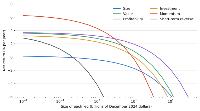
def break_even(f, idx):
    g = gross[f].loc[idx].mean()
    if g <= 0:
        return np.nan
    lo, hi = 1e6, 1e14
    for _ in range(60):
        mid = np.sqrt(lo * hi)
        lo, hi = (mid, hi) if impact_cost(port[f][1], mid).loc[idx].mean() < g else (lo, mid)
    return mid / 1e9

cap = pd.DataFrame({
    (per, col): [fn(f, idx) for f in FACTORS]
    for per, idx in (("1972-2025", full), ("2004-2024", recent))
    for col, fn in (("Cost, $1bn", lambda f, idx: 1200 * impact_cost(port[f][1], 1e9).loc[idx].mean()),
                    ("Cost, $10bn", lambda f, idx: 1200 * impact_cost(port[f][1], 1e10).loc[idx].mean()),
                    ("Break-even ($bn)", break_even))
}, index=list(FACTORS))
cap.apply(lambda c: c.map(lambda x: "" if pd.isna(x) else (f"{x:.3g}" if "Break" in c.name[1] else f"{x:.2f}")))| 1972-2025 | 2004-2024 | |||||
|---|---|---|---|---|---|---|
| Cost, $1bn | Cost, $10bn | Break-even ($bn) | Cost, $1bn | Cost, $10bn | Break-even ($bn) | |
| Size | 0.63 | 1.92 | 0.102 | 0.48 | 1.46 | |
| Value | 0.93 | 2.84 | 17.3 | 0.51 | 1.51 | 0.978 |
| Profitability | 0.60 | 1.82 | 43.8 | 0.32 | 0.95 | 148 |
| Investment | 1.07 | 3.26 | 10.5 | 0.66 | 1.98 | 2.36 |
| Momentum | 2.24 | 6.85 | 9.18 | 1.41 | 4.22 | 1.8 |
| Short-term reversal | 8.13 | 24.98 | 0.218 | 5.13 | 15.47 | 0.00428 |
Trading less
Figure 2 and Table 5 show what the factors could support. A fund with $1 billion in each leg pays 0.6 to 1.1 percentage points a year on the slow factors, 2.2 on momentum and 8.1 on short-term reversal. At $10 billion, the costs are about three times as large, as the square root implies. Over 1972 to 2025, the break-even size of each leg is $44 billion for profitability, $17 billion for value, $11 billion for investment and $9 billion for momentum, against $0.2 billion for short-term reversal and $0.1 billion for size, whose gross return is small. The ranking is the one Novy-Marx and Velikov (2016) find with spreads, and the sizes are those of large funds, as Frazzini et al. (2018) argue. Since 2004, with higher volume and lower gross returns, the break-even sizes fall to $1 billion to $2.4 billion for value, investment and momentum and to about $4 million for short-term reversal, while profitability, whose gross return held up, supports $148 billion.
Frazzini, Andrea, Ronen Israel, and Tobias J. Moskowitz. 2018. Trading Costs. Working paper. AQR Capital Management; Yale University.
The model was estimated on trades from 1998 to 2016. Applied to earlier years, it charges today’s costs on old returns, and costs were higher then: in Figure 6 of Frazzini et al. (2018), the impact of the same trade is higher from 1998 to 2005 than from 2006 to 2016.
Novy-Marx and Velikov (2016) find that the most effective way to trade less is a buy/hold spread, a stricter rule for entering a position than for keeping it. In Table 6, a stock enters a leg when it is in the outer third, as before, but stays until it leaves the outer half. Turnover falls by a quarter to a half: from 23% to 13% a month for momentum and from 71% to 55% for short-term reversal. The gross return of the other five factors falls too, since stocks stay in the portfolio after their signal has weakened, by about a percentage point a year for value and momentum. Whether the band pays depends on the cost. With the high-low spread, it raises the net return of momentum from 2.2% to 3.1% a year and reduces the loss of short-term reversal, but not enough to make it profitable. With TAQ spreads after 2004, it lowers the net return of value, profitability, investment and momentum, since the costs it saves are smaller than the return it gives up.
Novy-Marx, Robert, and Mihail Velikov. 2016. “A Taxonomy of Anomalies and Their Trading Costs.” Review of Financial Studies 29 (1): 104–47.
band = {f: trades(weights(stocks, c, s, band=(1 / 3, 1 / 2)), stocks) for f, (_, c, s) in FACTORS.items()}
rows = {}
for f in FACTORS:
    for name, (g, T) in (("Standard", port[f]), ("Band", band[f])):
        rows[f, name] = {
            ("1972-2025", "Turnover (%)"): 100 * turnover(T).loc[full].mean(),
            ("1972-2025", "Gross"): 1200 * g.loc[full].mean(),
            ("1972-2025", "Net, high-low"): 1200 * (g - spread_cost(T, "bidaskhl_21d")).loc[full].mean(),
            ("2004-2024", "Gross"): 1200 * g.loc[recent].mean(),
            ("2004-2024", "Net, TAQ"): 1200 * (g - spread_cost(T, "espread")).loc[recent].mean(),
        }
pd.DataFrame(rows).T.round(2)| 1972-2025 | 2004-2024 | |||||
|---|---|---|---|---|---|---|
| Turnover (%) | Gross | Net, high-low | Gross | Net, TAQ | ||
| Size | Standard | 5.91 | 0.22 | -1.20 | -1.88 | -2.12 |
| Band | 3.54 | 0.66 | -0.11 | -1.03 | -1.15 | |
| Value | Standard | 9.76 | 3.73 | 1.77 | 0.50 | 0.25 |
| Band | 5.10 | 2.69 | 1.64 | 0.22 | 0.09 | |
| Profitability | Standard | 7.13 | 3.76 | 2.31 | 3.57 | 3.39 |
| Band | 5.03 | 3.02 | 1.97 | 2.70 | 2.57 | |
| Investment | Standard | 11.51 | 3.35 | 1.20 | 0.99 | 0.71 |
| Band | 7.96 | 2.84 | 1.33 | 0.63 | 0.43 | |
| Momentum | Standard | 23.26 | 6.57 | 2.16 | 1.85 | 1.27 |
| Band | 13.26 | 5.72 | 3.13 | 1.30 | 0.95 | |
| Short-term reversal | Standard | 70.85 | 3.97 | -9.34 | 0.65 | -1.15 |
| Band | 54.63 | 3.68 | -6.61 | 0.67 | -0.71 | |
What we learned
How much an anomaly costs to trade depends first on how much it trades, and then on what a trade costs. Turnover ranges from 6% of each leg a month for size to 71% for short-term reversal. The cost per trade depends on how it is measured. Spreads estimated from daily high and low prices are 9 to 12 times the effective spreads in TAQ for large stocks, and they make momentum lose two thirds of its return to costs and short-term reversal lose money. With effective spreads, the same factors lose a seventh as much. Much of the disagreement in the literature comes from this measurement.
With effective spreads, the slow factors and momentum could be traded at the scale of large funds: over 1972 to 2025, the market impact model of Frazzini et al. (2018) gives break-even sizes of $9 billion to $44 billion in each leg. Short-term reversal breaks even at about $0.2 billion, and size, whose gross return is small, at less. Since 2004, though, the gross returns themselves have fallen, and only profitability earns more than 2% a year before costs. Net of costs, the expected returns of most of these factors are small, as Chen and Velikov (2023) find, mostly because the gross returns declined, not because of trading costs.
Frazzini, Andrea, Ronen Israel, and Tobias J. Moskowitz. 2018. Trading Costs. Working paper. AQR Capital Management; Yale University.
Chen, Andrew Y., and Mihail Velikov. 2023. “Zeroing in on the Expected Returns of Anomalies.” Journal of Financial and Quantitative Analysis 58 (3): 968–1004.
Building a factor to trade less, with a buy/hold band, pays when costs are high relative to the return given up, as for momentum with the high-low spreads. With today’s spreads it costs more return than it saves. Short-sale fees, which Chen and Velikov (2023) put at 10 to 20 bps a month, are not included here and would reduce the net returns of the short legs further.