import numpy as np
import pandas as pd
from threadpoolctl import threadpool_limits
from _portfolio import load_wrds, minvar_longonly_pgd, summarize

# Small matrices solve faster on a few threads than on all cores
threadpool_limits(4)

crsp_m = load_wrds("crsp_msf_1963_2025", """
    SELECT a.permno, a.date, a.ret, a.shrout, a.prc
    FROM crsp.msf AS a
    LEFT JOIN crsp.msenames AS b
      ON a.permno = b.permno
     AND b.namedt <= a.date
     AND a.date <= b.nameendt
    WHERE a.date BETWEEN '1963-01-01' AND '2025-12-31'
      AND b.exchcd BETWEEN 1 AND 3
      AND b.shrcd BETWEEN 10 AND 11
""")

crsp_vw = load_wrds("crsp_msi_1963_2025", """
    SELECT date, vwretd
    FROM crsp.msi
    WHERE date BETWEEN '1963-01-01' AND '2025-12-31'
""")

ff = load_wrds("ff_factors_monthly_1963_2025", """
    SELECT date, rf
    FROM ff.factors_monthly
    WHERE date BETWEEN '1963-01-01' AND '2025-12-31'
""")Minimum-Variance Portfolios from Daily Returns
Computed on October 9, 2026.
The previous notebook estimated the covariance matrix of 100 stocks from 60 monthly returns, so the sample matrix was singular. Its last section traced the difficulty to the complexity c = N / (T - 1), the number of stocks per direction the sample matrix can see, and found the unconstrained GMV portfolio riskiest just below c = 1. Daily returns give about 1,260 observations over the same five years, which takes c from 1.7 to 0.08 with 100 stocks. Here we form the same portfolios from daily covariance matrices and vary both the number of stocks N and the length of the estimation window. The question is whether daily data help because of their frequency or only because they lower c.
Data
Monthly returns, market capitalizations, the CRSP value-weighted index and the T-bill rate are the same as in the previous notebook. Daily returns come from crsp.dsf, pulled only for the stocks that are ever among the 500 largest at a formation date. CRSP data on WRDS, monthly and daily alike, end in December 2024, so the sample period is the same as in the previous notebook.
A stock is eligible at month t if it has a return in each of the 60 months ending at t, as before, whatever window is used for estimation. The universe is then the same at every window length, and only the estimate changes. The pivoted tables are rebuilt from a single array, which makes row lookups much faster.
def dense(df):
    return pd.DataFrame(df.to_numpy(dtype=float), index=df.index, columns=df.columns)

crsp_m["mcap"] = crsp_m["prc"].abs() * crsp_m["shrout"] / 1e6
rets  = dense(crsp_m.pivot(index="date", columns="permno", values="ret").sort_index())
mcaps = dense(crsp_m.pivot(index="date", columns="permno", values="mcap").reindex(rets.index))
mcaps = mcaps.where(rets.notna().rolling(60).sum() == 60)
mkt   = crsp_vw.set_index("date")["vwretd"].astype(float)
rf    = ff.set_index(ff["date"].dt.to_period("M"))["rf"].astype(float)

universe = set()
for t in range(59, len(rets) - 1):
    universe |= set(mcaps.iloc[t].dropna().nlargest(500).index)

crsp_d = load_wrds("crsp_dsf_top500_1963_2025", f"""
    SELECT permno, date, ret
    FROM crsp.dsf
    WHERE date BETWEEN '1963-01-01' AND '2025-12-31'
      AND permno IN ({", ".join(str(int(p)) for p in sorted(universe))})
""")
rets_d = dense(crsp_d.pivot(index="date", columns="permno", values="ret").sort_index())
Portfolio formation
form_portfolios works as in the previous notebook, except that the covariance matrix is estimated from est, either monthly or daily returns, over the est_months calendar months ending at t. A missing daily return, about 0.3% of the sample, is set to zero, which shrinks that stock’s variance and covariances slightly. T records the number of observations in each window. The GMV weights do not change when the covariance matrix is multiplied by a constant, so a daily estimate needs no conversion to monthly units before forming a portfolio held for a month. Daily covariances have one known bias: a stock that trades infrequently moves with the market a day late, which understates its daily covariances. Among the largest stocks this matters little.
The unconstrained portfolio uses the ridgeless rule of the previous notebook. It is the textbook portfolio when N < T - 1, and the minimum-norm portfolio with zero sample variance when N > T - 1.
def form_portfolios(rets, mcaps, est, rules, est_months=60, top_n=100):
    dates = rets.index
    out = {}
    for t in range(59, len(dates) - 1):
        dt, dt_next = dates[t], dates[t + 1]
        elig = mcaps.loc[dt].dropna().nlargest(top_n).index
        start = (dt.to_period("M") - est_months + 1).start_time
        X = est.loc[start:dt, elig].fillna(0.0)

        r_next = rets.loc[dt_next, elig].dropna()
        w_vw = mcaps.loc[dt, r_next.index]
        row = {"vw": (w_vw / w_vw.sum()) @ r_next, "T": len(X)}

        for name, rule in rules.items():
            w = pd.Series(rule(X), index=X.columns)
            w_next = w.reindex(r_next.index)
            row[name] = (w_next / w_next.sum()) @ r_next
            row[f"{name}_names"] = (w != 0).sum()
            row[f"{name}_gross"] = w.abs().sum()
        out[dt_next] = row
    port = pd.DataFrame(out).T.astype(float)
    port["mkt"] = mkt.reindex(port.index)
    port["rf"] = rf.reindex(port.index.to_period("M")).to_numpy()
    return port

def gmv_longonly(X):
    return minvar_longonly_pgd(X.cov().to_numpy())

def gmv_unconstrained(X):
    S = X.cov().to_numpy()
    z = 1e-8 * np.trace(S) / len(S)
    w = np.linalg.solve(S + z * np.eye(len(S)), np.ones(len(S)))
    return w / w.sum()

rules = {"lo": gmv_longonly, "un": gmv_unconstrained}
We run every combination of N = 50, 100, 250 and 500 with daily windows of 60, 24, 12 and 6 months, and monthly windows of 60 months as in the previous notebook. A month has about 21 trading days, so the daily windows have about 1,260, 504, 252 and 126 observations. This cell takes about 20 minutes.
sizes = [50, 100, 250, 500]
configs = ([("Monthly", 60, n) for n in sizes]
           + [("Daily", m, n) for m in (60, 24, 12, 6) for n in sizes])
ports = {(freq, m, n): form_portfolios(rets, mcaps, rets if freq == "Monthly" else rets_d,
                                       rules, est_months=m, top_n=n)
         for freq, m, n in configs}
Daily versus monthly estimates
fmt = lambda x: "" if pd.isna(x) else f"{round(x, 2) + 0.0:.2f}"
m, d = ports[("Monthly", 60, 100)], ports[("Daily", 60, 100)]
cols = {"Long-only, monthly": (m, "lo"), "Unconstrained, monthly": (m, "un"),
        "Long-only, daily": (d, "lo"), "Unconstrained, daily": (d, "un")}
tbl = pd.DataFrame({name: pd.concat([summarize(p[c], p["mkt"], p["rf"]),
                                     pd.Series({"Stocks held": p[f"{c}_names"].mean(),
                                                "Gross exposure": p[f"{c}_gross"].mean()})])
                    for name, (p, c) in cols.items()})
tbl["CRSP VW"] = summarize(d["mkt"], d["mkt"], d["rf"])
tbl.map(fmt)| Long-only, monthly | Unconstrained, monthly | Long-only, daily | Unconstrained, daily | CRSP VW | |
|---|---|---|---|---|---|
| Mean (%) | 10.52 | 9.17 | 10.54 | 10.53 | 10.95 |
| Volatility (%) | 12.38 | 16.36 | 11.98 | 11.90 | 15.77 |
| Sharpe ratio | 0.49 | 0.29 | 0.51 | 0.52 | 0.41 |
| Beta | 0.60 | 0.44 | 0.55 | 0.43 | 1.00 |
| Alpha (%) | 2.16 | 1.90 | 2.54 | 3.32 | 0.00 |
| Alpha p-value | 0.04 | 0.34 | 0.02 | 0.01 | |
| Max drawdown (%) | -38.66 | -56.18 | -34.05 | -36.71 | -51.48 |
| Stocks held | 15.75 | 100.00 | 23.31 | 100.00 | |
| Gross exposure | 1.00 | 5.53 | 1.00 | 3.04 |
The monthly columns reproduce the top-100 results of the previous notebook. Moving to daily data takes c from 1.69 to 0.08 and changes the unconstrained portfolio the most: its volatility falls from 16.4% to 11.9% and its Sharpe ratio rises from 0.29 to 0.52. It is no longer the riskiest portfolio. Its volatility matches the long-only portfolio’s, with a lower beta and a higher alpha. It holds every stock with gross exposure of about three, so each dollar of capital carries about a dollar of short positions that must be borrowed and rebalanced monthly. The long-only portfolio changes little, although daily estimates spread it over more stocks, 23 on average instead of 16.
Complexity, not frequency
Figure 1 places every configuration by its complexity. Two of them land on c = 1: 500 stocks with 24 months of daily data and 250 stocks with 12 months, where the number of stocks about equals the number of trading days.
import matplotlib.pyplot as plt
from matplotlib.ticker import NullLocator, StrMethodFormatter

grid = pd.DataFrame({k: {"T": p["T"].mean(),
                         "c": k[2] / (p["T"].mean() - 1),
                         "lo": 100 * np.sqrt(12) * p["lo"].std(),
                         "un": 100 * np.sqrt(12) * p["un"].std(),
                         "lo_names": p["lo_names"].mean(),
                         "un_gross": p["un_gross"].mean()}
                     for k, p in ports.items()}).T
grid.index.names = ["Data", "Window (months)", "N"]

fig, ax = plt.subplots(figsize=(8, 4.5))
for freq, marker in (("Daily", "o"), ("Monthly", "s")):
    g = grid.xs(freq)
    ax.scatter(g["c"], g["un"], marker=marker, s=50, color="#eb6834", label=f"Unconstrained, {freq.lower()}")
    ax.scatter(g["c"], g["lo"], marker=marker, s=50, color="#2a78d6", label=f"Long-only, {freq.lower()}")
ax.axvline(1, color="#888888", linestyle="--", linewidth=1)
ax.axhline(100 * np.sqrt(12) * d["mkt"].std(), color="#888888", linestyle=":", linewidth=1)
ax.set_xscale("log")
ax.set_yscale("log")
ax.xaxis.set_major_formatter(StrMethodFormatter("{x:g}"))
ax.yaxis.set_major_formatter(StrMethodFormatter("{x:g}"))
ax.yaxis.set_minor_locator(NullLocator())
ax.set_yticks([10, 20, 50, 100, 200, 500, 1000])
ax.set_xlabel("Complexity $c = N / (T - 1)$")
ax.set_ylabel("Volatility (%)")
ax.grid(axis="y", color="#e5e5e5", linewidth=0.8)
ax.spines[["top", "right"]].set_visible(False)
ax.legend(frameon=False)
plt.tight_layout()
plt.show()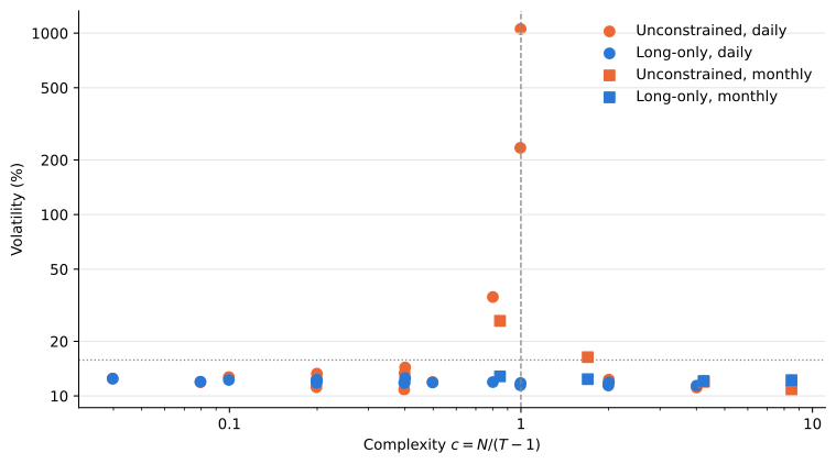
grid.rename(columns={"T": "Observations", "c": "Complexity", "lo": "Volatility, long-only (%)",
                     "un": "Volatility, unconstrained (%)", "lo_names": "Stocks held, long-only",
"un_gross": "Gross exposure, unconstrained"}).map(fmt)| Observations | Complexity | Volatility, long-only (%) | Volatility, unconstrained (%) | Stocks held, long-only | Gross exposure, unconstrained | |||
|---|---|---|---|---|---|---|---|---|
| Data | Window (months) | N | ||||||
| Monthly | 60 | 50 | 60.00 | 0.85 | 12.82 | 25.94 | 12.57 | 9.27 |
| 100 | 60.00 | 1.69 | 12.38 | 16.36 | 15.75 | 5.53 | ||
| 250 | 60.00 | 4.24 | 12.08 | 11.96 | 20.75 | 3.63 | ||
| 500 | 60.00 | 8.47 | 12.23 | 10.84 | 25.54 | 3.02 | ||
| Daily | 60 | 50 | 1258.53 | 0.04 | 12.45 | 12.47 | 17.08 | 2.43 |
| 100 | 1258.53 | 0.08 | 11.98 | 11.90 | 23.31 | 3.04 | ||
| 250 | 1258.53 | 0.20 | 12.02 | 11.18 | 35.74 | 4.39 | ||
| 500 | 1258.53 | 0.40 | 11.80 | 10.84 | 48.16 | 6.06 | ||
| 24 | 50 | 503.37 | 0.10 | 12.25 | 12.70 | 16.92 | 2.64 | |
| 100 | 503.37 | 0.20 | 11.80 | 12.34 | 22.70 | 3.45 | ||
| 250 | 503.37 | 0.50 | 11.87 | 11.92 | 33.36 | 6.06 | ||
| 500 | 503.37 | 1.00 | 11.45 | 233.25 | 44.92 | 68.76 | ||
| 12 | 50 | 251.68 | 0.20 | 12.29 | 13.27 | 16.10 | 2.92 | |
| 100 | 251.68 | 0.40 | 11.84 | 13.35 | 21.49 | 4.21 | ||
| 250 | 251.68 | 1.00 | 11.78 | 1054.48 | 31.65 | 62.16 | ||
| 500 | 251.68 | 1.99 | 11.42 | 11.72 | 42.43 | 5.60 | ||
| 6 | 50 | 125.84 | 0.40 | 12.54 | 14.35 | 14.96 | 3.65 | |
| 100 | 125.84 | 0.80 | 11.92 | 35.11 | 19.74 | 7.99 | ||
| 250 | 125.84 | 2.00 | 11.87 | 12.30 | 28.35 | 4.91 | ||
| 500 | 125.84 | 4.01 | 11.39 | 11.12 | 36.42 | 3.44 |
The unconstrained portfolio’s volatility depends mostly on c, not on the data frequency. Monthly and daily points fall on roughly the same curve, which peaks at c = 1 and falls on either side, the pattern Hellum et al. (2026) derive for the GMV portfolio. Points with the same c still differ: at c = 0.4 volatility ranges from 10.8% with 500 stocks and 60 months to 14.4% with 50 stocks and 6 months, so N and the window length matter beyond their ratio.
The peak has a simple cause. As N approaches T - 1, the smallest eigenvalues of the sample matrix approach zero, and inverting it puts the largest weights on the directions that look almost riskless in the sample, which are mostly noise. At c = 1 the unconstrained portfolio has gross exposure of 62 to 69 and volatility of 233% and 1,054%. Past c = 1 the ridgeless rule picks the riskless-in-sample portfolio closest to equal weights, as in the previous notebook, and the weights settle down again. The long-only portfolio’s volatility barely changes across the grid, staying between 11.4% and 12.8%, because the constraint rules out the large offsetting positions that the near-zero eigenvalues call for.
What we learned
Daily data solve the problem of the previous notebook mainly because they lower c. A short daily window or a large universe brings back the same peak at c = 1. With c at 0.2 or below, or at 2 or above, the unconstrained portfolio’s volatility is within about 1.5 percentage points of the long-only portfolio’s, and below it in the most complex case. The damage is not confined to c = 1: at c = 0.8 volatility is already 35%, and at c = 0.4 the unconstrained portfolio can be nearly two points riskier than the long-only one. An investor can compute c in advance, but avoiding the peak means staying well away from it, and even then the unconstrained portfolio holds every stock with gross exposure of at least 2.4. The long-only portfolio delivers about the same volatility everywhere on the grid without them, which makes the constraint insurance against landing near c = 1.
Low and high complexity give about the same volatility here. With 500 stocks the unconstrained portfolio has a volatility of 10.8% both from 60 months of daily data (c = 0.4) and from monthly data (c = 8.5). Daily data reach low complexity without giving up stocks, but only for the covariance matrix. The precision of an estimated mean depends on the length of the sample in calendar time, not on how often returns are observed (Merton 1980), so for expected returns c stays high however fine the data. High complexity also matters when daily returns are not available, or when covariances change over time and call for short windows. Hellum et al. (2026) estimate portfolios of 153 factors from 12 monthly observations, where low complexity means a dozen assets at most, and find that the GMV portfolio at c \gg 1 has about half the volatility of the best one at c < 1. With daily returns on large stocks, low complexity no longer means few assets, and the advantage of high complexity disappears.
Merton, Robert C. 1980. “On Estimating the Expected Return on the Market: An Exploratory Investigation.” Journal of Financial Economics 8 (4): 323–61.
Hellum, Oliver, Theis I. Jensen, Bryan T. Kelly, and Semyon Malamud. 2026. Complex Modern Portfolio Theory. Working Paper No. 35246. National Bureau of Economic Research.