import urllib.request
import numpy as np
import pandas as pd
import matplotlib.pyplot as plt
from matplotlib.ticker import FixedLocator, NullLocator, StrMethodFormatter
from threadpoolctl import threadpool_limits
from _portfolio import DATA_DIR, load_wrds, load_jkp, sharpe, summarize, factor_regression

threadpool_limits(4)

jkp = load_jkp("jkp_usa_all_factors_monthly_vw_cap",
               "https://jkpfactors-data.s3.amazonaws.com/public/"
               "%5Busa%5D_%5Ball_factors%5D_%5Bmonthly%5D_%5Bvw_cap%5D.zip")

def load_details(url, file=DATA_DIR / "jkp_factor_details.xlsx"):
    if not file.exists():
        file.write_bytes(urllib.request.urlopen(url).read())
    return pd.read_excel(file, engine="openpyxl")

details = load_details("https://raw.githubusercontent.com/bkelly-lab/ReplicationCrisis/"
                       "master/GlobalFactors/Factor%20Details.xlsx")

ff = load_wrds("ff_factors_monthly_1963_2025", """
    SELECT date, rf
    FROM ff.factors_monthly
    WHERE date BETWEEN '1963-01-01' AND '2025-12-31'
""")

ff5 = load_wrds("ff_fivefactors_monthly_1963_2025", """
    SELECT date, mktrf, smb, hml, rmw, cma, umd
    FROM ff.fivefactors_monthly
    WHERE date BETWEEN '1963-01-01' AND '2025-12-31'
""")

F = jkp.pivot(index="date", columns="name", values="ret")
F.index = F.index.to_period("M")
F = F.loc[F.notna().all(axis=1).idxmax():]
ff6 = ff5.set_index(ff5["date"].dt.to_period("M")).drop(columns="date").astype(float)
rf = ff.set_index(ff["date"].dt.to_period("M"))["rf"].astype(float)

# Original sample period and publication year of each factor
d = details[details["abr_jkp"].isin(F.columns)].set_index("abr_jkp").reindex(F.columns)
years = d["in-sample period"].astype(str).str.findall(r"(?:19|20)\d\d")
info = pd.DataFrame({"start": years.str[0].astype(int), "end": years.str[-1].astype(int),
                     "pub": d["cite"].str.extract(r"((?:19|20)\d\d)", expand=False).astype(float)})
info.loc[["op_at", "cop_at"], "pub"] = [2015, 2016]
info["pub"] = info["pub"].fillna(2020).astype(int)

def published(month):
    return info["pub"].to_numpy() < month.year

oos = pd.period_range("1992-01", "2025-12", freq="M")The Factor Zoo in Real Time
The SDF of An SDF for the Factor Zoo earned an out-of-sample Sharpe ratio near 2 from 1992 to 2025, most of it before 2005. Out of sample meant that the weights of each month used only past returns. The menu of factors did not: all 153 factors entered from 1992 on, although most of them had not yet been published. An investor in 1992 could not have traded a factor that no one had documented, and many of the factors were discovered with data that overlap our sample. That notebook ended with the question of whether the decline after 2005 reflects publication, the selection of the factors, or both.
Two lines of research bear on it. McLean and Pontiff (2016) follow 97 predictors of stock returns after the study that documented them. Their returns are 26% lower after the end of the original sample, an upper bound on what was a statistical fluke, and 58% lower after publication, when investors learn about them. Harvey et al. (2016) argue that with hundreds of characteristics tested, many published factors are false discoveries. Both say that a factor’s returns before its publication overstate what an investor can expect from it.
Harvey, Campbell R., Yan Liu, and Heqing Zhu. 2016“... And the Cross-Section of Expected Returns.” The Review of Financial Studies 29 (1): 5–68.
This notebook builds the SDF that an investor could have held at the time. Each month, the menu contains only the factors already published. The estimation is the same as before, so any difference comes from the menu alone.
Data
The factor returns are those of the previous notebooks, the 153 U.S. factors of Jensen et al. (2023) with returns from November 1971 to December 2025. Their documentation lists, for each factor, the study that introduced it and the sample period of that study. The publication year is the year in the citation, which is the year of the journal issue. Eleven factors have no citation. Two are the operating profitability measures of Ball et al. (2015) and Ball et al. (2016), which we date to those papers. The other nine have sample periods that end in 2016, the end of the sample of Hou et al. (2020), whose list of anomalies the documentation follows. We date them to 2020, the year Hou et al. (2020) was published, which can only delay their entry.
Ball, Ray, Joseph Gerakos, Juhani T. Linnainmaa, and Valeri V. Nikolaev. 2015. “Deflating Profitability.” Journal of Financial Economics 117 (2): 225–48.
Ball, Ray, Joseph Gerakos, Juhani T. Linnainmaa, and Valeri V. Nikolaev. 2016. “Accruals, Cash Flows, and Operating Profitability in the Cross Section of Stock Returns.” Journal of Financial Economics 121 (1): 28–45.
Hou, Kewei, Chen Xue, and Lu Zhang. 2020. “Replicating Anomalies.” Review of Financial Studies 33 (5): 2019–133.
McLean and Pontiff (2016) date publication by the year and month on the journal’s cover. With only the year, we count a factor as published from January of the following year. A factor enters the menu of month t if its publication year is earlier than the year of t. Its whole history then becomes available, including the returns before publication, since an investor who reads the study can rebuild the factor from the start of the data.
Figure 1 shows how the menu grows. In January 1992, when the out-of-sample period of the previous notebooks starts, 11 of the 153 factors had been published. By 2005 there were 57, and the last ones enter in 2021. The median factor was published in 2006, so for half of the out-of-sample period the hindsight SDF held mostly factors that did not yet exist in the literature.
yrs = np.arange(1972, 2026)
count = [(info["pub"] < y).sum() for y in yrs]
fig, ax = plt.subplots(figsize=(8, 3.5))
ax.axvspan(1992, 2025, color="#eeeeee", linewidth=0)
ax.step(yrs, count, where="post", color="#2a78d6", linewidth=1.8)
ax.set_xlabel("Year")
ax.set_ylabel("Published factors")
ax.set_ylim(0, 160)
ax.grid(axis="y", color="#e5e5e5", linewidth=0.8)
ax.spines[["top", "right"]].set_visible(False)
plt.tight_layout()
plt.show()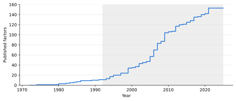
Jensen, Theis Ingerslev, Bryan Kelly, and Lasse Heje Pedersen. 2023. “Is There a Replication Crisis in Finance?” The Journal of Finance 78 (5): 2465–518.
Returns before and after publication
We first repeat the regression of McLean and Pontiff (2016) with these factors. For factor i in month t,
R_{it} = \alpha_i + \beta_1 \, \text{Post-sample}_{it} + \beta_2 \, \text{Post-publication}_{it} + e_{it}, \tag{1}
where Post-sample is one after the end of the original study’s sample and up to its publication year, and Post-publication is one after the publication year. The fixed effect \alpha_i absorbs each factor’s average return in the original sample, and months before the original sample starts are dropped. Standard errors are clustered by month, since factor returns are correlated within a month. Dividing \beta_1 and \beta_2 by the average in-sample return gives the proportional declines that McLean and Pontiff (2016) report.
rows = []
y = F.index.year
for f in F.columns:
    s, e, p = info.loc[f, ["start", "end", "pub"]]
    keep = y >= s
    rows.append(pd.DataFrame({"factor": f, "month": F.index[keep], "ret": 100 * F[f].to_numpy()[keep],
                              "post_sample": ((y > e) & (y <= p))[keep], "post_pub": (y > p)[keep]}))
panel = pd.concat(rows, ignore_index=True)

def within(x):
    return (x - x.groupby(panel["factor"]).transform("mean")).to_numpy()

X = np.column_stack([within(panel[c].astype(float)) for c in ("post_sample", "post_pub")])
yv = within(panel["ret"])
b = np.linalg.lstsq(X, yv, rcond=None)[0]
u = X * (yv - X @ b)[:, None]
G = pd.DataFrame(u).groupby(panel["month"].to_numpy()).sum().to_numpy()
XtX_inv = np.linalg.inv(X.T @ X)
se = np.sqrt(np.diag(XtX_inv @ G.T @ G @ XtX_inv))
in_mean = panel[~panel["post_sample"] & ~panel["post_pub"]].groupby("factor")["ret"].mean().mean()

decay = pd.DataFrame({"Coefficient": b, "Standard error": se, "Share of in-sample mean": b / in_mean},
                     index=["Post-sample", "Post-publication"])
decay.loc["In-sample mean"] = [in_mean, np.nan, np.nan]
decay.round(3)| Coefficient | Standard error | Share of in-sample mean | |
|---|---|---|---|
| Post-sample | -0.032 | 0.047 | -0.115 |
| Post-publication | -0.171 | 0.061 | -0.609 |
| In-sample mean | 0.281 | NaN | NaN |
In their original samples the factors earned 0.28% a month on average. After the sample ended but before publication, returns were 0.03 percentage points lower, a decline of 12% that is smaller than its standard error. After publication they were 0.17 percentage points lower, a decline of 61% with a t-statistic of 2.8. McLean and Pontiff (2016) find 26% and 58% for their 97 predictors. The decline after publication is almost the same, while the decline before it is smaller here, so little of the original returns looks like a statistical fluke and most of the decay comes with publication. Either way, a factor’s history before its publication overstates what an investor could expect from it afterward, and the hindsight SDF puts those years in its out-of-sample period.
The SDF in real time
The estimator is the ridge SDF of An SDF for the Factor Zoo. Each month we take the past T months of returns of the factors on the menu, compute
w(z) = \Big(\frac{1}{T} \sum_{s} F_s F_s^\top + z \bar{\lambda} I\Big)^{-1} \bar{F}
for a grid of penalties z, scale the weights to a gross exposure of one, and record the next month’s return. The hindsight SDF uses all 153 factors every month and reproduces the previous notebook. The real-time SDF uses only the factors published before that year, so the number of factors N grows from 11 in 1992 to 153. Since the penalty is a multiple z of the average eigenvalue, the same z shrinks the estimate by a comparable amount whatever the size of the menu.
zs = np.r_[0.0, 10.0 ** np.arange(-4, 1.01, 0.5)]

def ridge_sdf(X, zs):
    T, N = X.shape
    mu = X.mean(axis=0)
    _, s, Vt = np.linalg.svd(X / np.sqrt(T), full_matrices=False)
    lam = s ** 2
    keep = lam > 1e-10 * lam.max()
    lam, Vt = lam[keep], Vt[keep]
    m = Vt @ mu
    scale = (s ** 2).sum() / N
    W = []
    for z in zs:
        if z == 0:
            w = Vt.T @ (m / lam)
        else:
            a = z * scale
            w = Vt.T @ (m / (lam + a)) + (mu - Vt.T @ m) / a
        W.append(w / np.abs(w).sum())
    return np.array(W)

def sdf_returns(F, T, zs, menu=None):
    # menu(month) gives the factors available in that month; None means all of them
    X, idx = F.to_numpy(), F.index
    R = []
    for t in range(T, len(idx)):
        cols = np.ones(X.shape[1], bool) if menu is None else menu(idx[t])
        R.append(ridge_sdf(X[t - T:t, cols], zs) @ X[t, cols])
    return pd.DataFrame(R, index=idx[T:], columns=zs)

def select_z(R, burn=60):
    # Each month, the z with the highest Sharpe ratio on past out-of-sample returns
    sr = (R.expanding(burn).mean() / R.expanding(burn).std()).shift(1).dropna(how="all")
    best = sr.idxmax(axis=1)
    return pd.Series([R.at[t, z] for t, z in best.items()], index=best.index), best

windows = [60, 120, 240]
menus = {"Hindsight": None, "Real time": published}
R = {(m, T): sdf_returns(F, T, zs, menu) for m, menu in menus.items() for T in windows}
sr_z = pd.DataFrame({(m, T): sharpe(R[m, T].loc[oos]) for m, T in R})
sr_z.index.name = "z"
x0 = zs[1] / 10 ** 0.75
xs = np.r_[x0, zs[1:]]
fig, ax = plt.subplots(figsize=(8, 4.5))
for T, col in zip((120, 240), ("#2a78d6", "#3a9e5c")):
for m, ls, mk in (("Hindsight", "-", "o"), ("Real time", "--", "s")):
ax.plot(xs[1:], sr_z[m, T].iloc[1:], color=col, linestyle=ls, marker=mk, ms=4, label=f"{m}, T = {T}")
ax.scatter([x0], [sr_z[m, T].iloc[0]], color=col, marker=mk, s=30)
ax.set_xscale("log")
ax.xaxis.set_major_locator(FixedLocator([x0, 1e-4, 1e-3, 1e-2, 1e-1, 1, 10]))
ax.xaxis.set_minor_locator(NullLocator())
ax.set_xticklabels(["0", "$10^{-4}$", "$10^{-3}$", "$10^{-2}$", "$10^{-1}$", "1", "10"])
ax.set_xlabel("Ridge penalty $z$")
ax.set_ylabel("Sharpe ratio")
ax.grid(axis="y", color="#e5e5e5", linewidth=0.8)
ax.spines[["top", "right"]].set_visible(False)
ax.legend(frameon=False, ncol=2)
plt.tight_layout()
plt.show()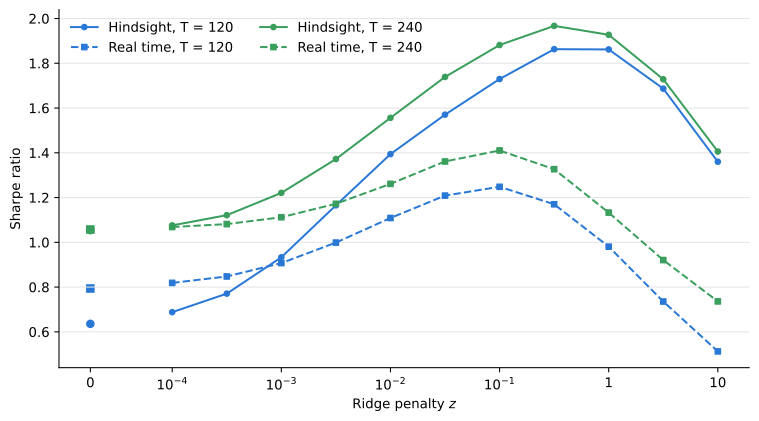
sr_z.round(2)The real-time menu costs about 30% of the Sharpe ratio. At the best penalty, the hindsight SDF reaches 1.67, 1.86 and 1.97 with windows of 60, 120 and 240 months, and the real-time SDF 1.21, 1.25 and 1.41. Without shrinkage the two are close: the real-time SDF earns 1.06 against 1.05 with 240 months, and is even ahead with 120 months, 0.79 against 0.64. Almost all of the difference comes from what shrinkage adds. With the full menu, the penalty raises the Sharpe ratio by 0.66 to 1.22; with the real-time menu, by 0.35 to 0.46. The best penalty is also smaller, z = 0.1 instead of 0.32, and the Sharpe ratio falls faster for large penalties. As z grows the weights approach the past average returns, and with a small menu that means a few concentrated bets.
Performance
As in the previous notebook, an investor has to choose the penalty with past data. Each month, select_z picks the z with the highest Sharpe ratio on past out-of-sample returns, after a burn-in of 60 months, for windows of 60 and 120 months, whose returns start early enough for this history to be available by 1992. In the real-time SDF the burn-in itself uses only the factors published at the time, a handful in the early 1980s. The benchmarks are the market and 1/N across the published factors, which needs no estimation. Each strategy is scaled after the fact to the market’s volatility over 1992 to 2025, which leaves Sharpe ratios, betas, t-statistics and R^2 unchanged.
fmt = lambda x: "" if pd.isna(x) else f"{round(x, 2) + 0.0:.2f}"
cv = {(m, T): select_z(R[m, T]) for m in menus for T in (60, 120)}

strategies = {
    "1/N, real time": pd.Series([F.loc[t, published(t)].mean() for t in oos], index=oos),
    **{f"{m}, T = {T}": cv[m, T][0] for m in menus for T in (60, 120)},
}
mkt_ex, rf_o = ff6.loc[oos, "mktrf"], rf.loc[oos]
vol = mkt_ex.std()

def stats(ex):
    ex = ex.loc[oos] * vol / ex.loc[oos].std()
    coef, p, r2 = factor_regression(ex + rf_o, rf_o, ff6.loc[oos])
    return pd.concat([summarize(ex + rf_o, mkt_ex + rf_o, rf_o),
                      pd.Series({"FF6 alpha (%)": 1200 * coef[0], "FF6 alpha p-value": p[0], "FF6 R2": r2})])

tbl = pd.DataFrame({name: stats(ex) for name, ex in strategies.items()})
tbl.insert(0, "Market", summarize(mkt_ex + rf_o, mkt_ex + rf_o, rf_o))
tbl.map(fmt)| Market | 1/N, real time | Hindsight, T = 60 | Hindsight, T = 120 | Real time, T = 60 | Real time, T = 120 | |
|---|---|---|---|---|---|---|
| Mean (%) | 11.44 | 10.24 | 27.45 | 29.84 | 8.44 | 21.62 |
| Volatility (%) | 15.05 | 15.09 | 15.22 | 15.18 | 15.09 | 15.14 |
| Sharpe ratio | 0.60 | 0.52 | 1.66 | 1.82 | 0.40 | 1.27 |
| Beta | 1.00 | -0.53 | -0.06 | -0.11 | -0.06 | -0.02 |
| Alpha (%) | 0.00 | 12.54 | 25.55 | 28.38 | 6.53 | 19.38 |
| Alpha p-value | 0.00 | 0.00 | 0.00 | 0.01 | 0.00 | |
| Max drawdown (%) | -50.31 | -53.85 | -16.42 | -18.44 | -51.72 | -15.71 |
| FF6 alpha (%) | 4.74 | 21.68 | 23.96 | 4.43 | 16.52 | |
| FF6 alpha p-value | 0.00 | 0.00 | 0.00 | 0.05 | 0.00 | |
| FF6 R2 | 0.81 | 0.11 | 0.12 | 0.30 | 0.06 |
With 120 months, the real-time SDF has a Sharpe ratio of 1.27, against 1.82 for the hindsight SDF, and an FF6 alpha of 17% a year at the market’s volatility, against 24%. Both have market betas close to zero and drawdowns of 16% to 18%. The real-time SDF is still more than twice as good as the market by its Sharpe ratio, so the conclusion of the previous notebook survives, at a smaller scale.
With 60 months, choosing the penalty in real time fails. The history used to choose the penalty starts in the late 1970s, when the menu held a handful of factors, and it favored large penalties: the selection picks z = 1 or more in 342 of the 408 months. Large penalties make the weights close to proportional to past average returns. In early 2000, after the technology rally, that meant long momentum and short value, and in March 2000 the momentum factors lost 16% to 17% while the value factors gained 21% to 25%. The strategy lost 8.9% that month before scaling and has a maximum drawdown of 52%. Its Sharpe ratio over the whole period, 0.40, is lower than in each of the subperiods of Table 4, which can happen because its volatility changes with the selected penalty. The fixed penalty z = 0.1 would have given 1.21 with the same window, so the problem is the selection, not the estimator. With all 153 factors, the selection of the previous notebook stayed among three neighboring values around z = 0.32.
The 1/N portfolio of the published factors has a Sharpe ratio of 0.52, below the market’s, with a market beta of -0.53. Most of its return is explained by the six Fama-French factors (R^2 of 0.81), as one would expect of an average of published anomalies.
Subperiods
The previous notebook found that the SDF earned most of its Sharpe ratio before 2005 and attributed the decline to publication and to the selection of the factors. If the decline comes from the menu, the real-time SDF should show less of it. Table 4 splits the sample at the same dates.
periods = {"1992-2004": ("1992-01", "2004-12"), "2005-2014": ("2005-01", "2014-12"),
           "2015-2025": ("2015-01", "2025-12"), "1992-2025": ("1992-01", "2025-12")}
sub = pd.DataFrame({p: {name: sharpe(ex.loc[a:b]) for name, ex in {"Market": mkt_ex, **strategies}.items()}
                    for p, (a, b) in periods.items()})
sub.map(fmt)| 1992-2004 | 2005-2014 | 2015-2025 | 1992-2025 | |
|---|---|---|---|---|
| Market | 0.52 | 0.50 | 0.76 | 0.60 |
| 1/N, real time | 0.66 | 0.58 | 0.34 | 0.52 |
| Hindsight, T = 60 | 2.74 | 1.09 | 0.76 | 1.66 |
| Hindsight, T = 120 | 2.87 | 1.26 | 1.04 | 1.82 |
| Real time, T = 60 | 0.45 | 0.64 | 0.82 | 0.40 |
| Real time, T = 120 | 1.74 | 1.05 | 0.90 | 1.27 |
The gap between the two SDFs is concentrated in the early years. With 120 months, the hindsight SDF has a Sharpe ratio of 2.87 from 1992 to 2004, and the real-time SDF 1.74. From 2005 to 2014 the two earn 1.26 and 1.05, and from 2015 to 2025 1.04 and 0.90. The real-time SDF still declines, from 1.74 to 0.90, but by less than half as much as the hindsight SDF, and since 2015 it remains above the market’s 0.76. Most of what looked like a collapse after 2005 was the menu: the hindsight SDF held, in the 1990s, factors whose discovery was still to come.
The hindsight SDF can be split by the same dates. Each month, its return is the sum of the returns of its positions in factors already published and in factors not yet published. Table 5 shows how much of its average return came from each, with the penalty z = 0.32 that was best after the fact.
z_best = zs[8]

def split_returns(F, T, z):
    X, idx = F.to_numpy(), F.index
    rows = []
    for t in range(idx.get_loc(oos[0]), len(idx)):
        w = ridge_sdf(X[t - T:t], [z])[0]
        pub_t = published(idx[t])
        rows.append([w[pub_t] @ X[t, pub_t], w[~pub_t] @ X[t, ~pub_t]])
    return pd.DataFrame(rows, index=idx[idx.get_loc(oos[0]):], columns=["Published", "Not yet published"])

parts = split_returns(F, 120, z_best)
split = pd.DataFrame({p: 1200 * parts.loc[a:b].mean() for p, (a, b) in periods.items()}).T
split["Not yet published, share"] = split["Not yet published"] / split.sum(axis=1)
split.round(2)| Published | Not yet published | Not yet published, share | |
|---|---|---|---|
| 1992-2004 | 0.52 | 2.59 | 0.83 |
| 2005-2014 | 0.57 | 0.51 | 0.47 |
| 2015-2025 | 0.72 | 0.02 | 0.03 |
| 1992-2025 | 0.60 | 1.15 | 0.66 |
From 1992 to 2004, 83% of the hindsight SDF’s average return came from factors that had not yet been published. The share falls to 47% from 2005 to 2014 and 3% from 2015 to 2025, when nearly all factors had been published. The positions in published factors did not decline, earning 0.52% to 0.72% a year per unit of gross exposure. The decline of the hindsight SDF is therefore a decline in the returns of factors before their publication, which is the pattern McLean and Pontiff (2016) document factor by factor.
What we learned
The hindsight SDF of the previous notebook used factors before anyone had documented them. Restricting it to the factors published at the time lowers its Sharpe ratio from about 1.9 to about 1.3, with the same estimator and the same windows. The loss is concentrated before 2005, when most factors were still unpublished, and it accounts for more than half of the decline that the previous notebook found. Within the hindsight SDF, the positions in published factors did not decline; what fell was the return of factors before their publication.
The factor returns themselves agree. Regressed on the dates of their original samples and publication, the 153 factors earn 61% less after publication, close to the 58% of McLean and Pontiff (2016), and only 12% less between the end of the sample and publication. Publication matters more than data mining in these factors, although the factors here are those that Jensen et al. (2023) could replicate, which is itself a selection.
McLean, R. David, and Jeffrey Pontiff. 2016. “Does Academic Research Destroy Stock Return Predictability?” The Journal of Finance 71 (1): 5–32.
Jensen, Theis Ingerslev, Bryan Kelly, and Lasse Heje Pedersen. 2023. “Is There a Replication Crisis in Finance?” The Journal of Finance 78 (5): 2465–518.
The real-time SDF still has a Sharpe ratio of 1.27 and an FF6 alpha of 17% a year at the market’s volatility, before trading costs. Shrinkage helps less with a small menu, and choosing the penalty from a short history can fail badly, as it did in March 2000. The menu of factors is a choice made with hindsight as much as the weights are, and an out-of-sample test has to date both.