import numpy as np
import pandas as pd
import matplotlib.pyplot as plt
from threadpoolctl import threadpool_limits
from _portfolio import load_wrds, minvar_longonly_pgd

# Small matrices solve faster on one thread than on all cores
threadpool_limits(1)

crsp_m = load_wrds("crsp_msf_1963_2025", """
    SELECT permno, mthcaldt AS date, mthret AS ret, shrout, mthprc AS prc, mthcap
    FROM crsp.msf_v2
    WHERE mthcaldt BETWEEN '1963-01-01' AND '2025-12-31'
      AND sharetype = 'NS' AND securitytype = 'EQTY'
      AND securitysubtype = 'COM' AND usincflg = 'Y'
      AND issuertype IN ('ACOR', 'CORP')
      AND primaryexch IN ('N', 'A', 'Q')
      AND conditionaltype IN ('RW', 'NW')
""")

crsp_vw = load_wrds("crsp_msi_1963_2025", """
    SELECT mthcaldt AS date, mthtotret AS vwretd
    FROM crsp.indmthseriesdata
    WHERE indno = 1000200
      AND mthcaldt BETWEEN '1963-01-01' AND '2025-12-31'
""")

ff = load_wrds("ff_factors_monthly_1963_2025", """
    SELECT date, rf
    FROM ff.factors_monthly
    WHERE date BETWEEN '1963-01-01' AND '2025-12-31'
""")Can Regression Alphas Beat the CAPM?
The single index model regresses each stock’s excess return on the market’s. The intercept is the stock’s alpha, which the CAPM says is zero. An investor who believes the regressions keeps the estimated alphas and holds the tangency portfolio they imply, as in Treynor and Black (1973). An investor who believes the CAPM sets the alphas to zero. This notebook runs both investors on the 100 largest U.S. stocks from 1973 to 2025, each month with the previous ten years of returns.
The regression investor loses. The estimated alphas are noise, and the optimizer bets on it: the investor expects a Sharpe ratio between 2 and 10 every month and earns 0.04 or 0.06, significantly less than the market’s 0.45. The size of that error can be predicted before seeing any data, and ten years of returns are far too few to overcome it. The CAPM investor earns 0.43, about the market’s Sharpe ratio, which is all the CAPM promises. Estimation Error in the Tangency Portfolio shows the same result in simulations, where the truth is known, and shows also that the index model’s covariance matrix is valuable to an investor whose alphas come from somewhere other than past returns.
Pulling data from WRDS
The data are those of Implementing the Minimum-Variance Portfolio: monthly returns of common shares of U.S. companies on the NYSE, AMEX or Nasdaq from crsp.msf_v2, the CRSP value-weighted index as the market, and the one-month T-bill rate from ff. Each table is saved as a parquet file in _data on the first run. Delete a file to pull it again. The data loader and the long-only solver come from _portfolio.py, which must sit in the same folder as the notebook.
Market capitalization is in billions of dollars. The Fama-French file dates months by their first day and CRSP by the last trading day, so the T-bill rate is matched by calendar month. Everything below works with returns in excess of the T-bill rate.
crsp_m["mcap"] = crsp_m["prc"].abs() * crsp_m["shrout"] / 1e6
rets  = crsp_m.pivot(index="date", columns="permno", values="ret").sort_index().astype(float)
mcaps = crsp_m.pivot(index="date", columns="permno", values="mcap").reindex(rets.index).astype(float)
dates = rets.index
mkt = crsp_vw.set_index("date")["vwretd"].astype(float).reindex(dates)
rf  = pd.Series(ff.set_index(ff["date"].dt.to_period("M"))["rf"].astype(float)
                .reindex(dates.to_period("M")).to_numpy(), index=dates)

# Excess returns of the stocks and the market
xr = rets.sub(rf, axis=0)
xm = mkt - rf
Alphas and the tangency portfolio
With N stocks, the tangency portfolio puts weights w \propto \Sigma^{-1}\mu in the stocks and the rest of the capital in T-bills, where \mu is the vector of expected excess returns and \Sigma the covariance matrix. Its squared Sharpe ratio is \mu^\top\Sigma^{-1}\mu. Scaling w changes the portfolio’s risk but not its Sharpe ratio, so only the direction of \Sigma^{-1}\mu matters.
The single index model writes each stock’s excess return as R_i = \alpha_i + \beta_i R_M + e_i, with residuals uncorrelated with the market and with each other, so that \mu = \alpha + \beta\,\mu_M, \qquad \Sigma = \sigma_M^2\,\beta\beta^\top + D, where \mu_M and \sigma_M^2 are the market’s expected excess return and variance and D is the diagonal matrix of residual variances \sigma^2(e_i). The Sherman-Morrison formula inverts \Sigma in closed form, \Sigma^{-1} = D^{-1} - \frac{\sigma_M^2\, D^{-1}\beta\beta^\top D^{-1}}{1 + \sigma_M^2\, \beta^\top D^{-1}\beta}, \qquad \text{so} \qquad \Sigma^{-1}\mu = D^{-1}\alpha + \frac{\mu_M - \sigma_M^2\,\beta^\top D^{-1}\alpha}{1 + \sigma_M^2\, \beta^\top D^{-1}\beta}\, D^{-1}\beta. This is the decomposition of Treynor and Black (1973): an active portfolio with weights \alpha_i/\sigma^2(e_i), each alpha per unit of the residual risk it takes, and a passive portfolio with weights \beta_i/\sigma^2(e_i).
Treynor, Jack L., and Fischer Black. 1973. “How to Use Security Analysis to Improve Portfolio Selection.” Journal of Business 46 (1): 66–86.
With no alphas, only the passive portfolio is left, w_i \propto \operatorname{sign}(\mu_M)\,\beta_i/\sigma^2(e_i). Each stock’s weight is its beta per unit of residual variance, which makes this the portfolio of the N stocks most correlated with the market. With no alphas there is nothing to buy except market risk, and this portfolio buys it with the least firm-specific risk. In Treynor and Black (1973) the investor with no alphas holds the market itself, and here, where the market is not one of the assets, the portfolio closest to it takes its place. Only the sign of the market premium is left, and when the premium and all betas are positive, the portfolio is long-only without any constraint.
The investor does not know \alpha, \beta, D or \mu_M. Regressions of each stock’s excess return on the market’s over the estimation window give \hat\alpha_i, \hat\beta_i and \hat\sigma^2(e_i). The intercept of a regression satisfies \hat\alpha_i = \bar R_i - \hat\beta_i \bar R_M, so the regression investor, who keeps the estimated alphas, uses expected returns
\hat\mu_i = \hat\alpha_i + \hat\beta_i\,\bar R_M = \bar R_i,
the sample means. Keeping the regression alphas is the same as using sample means, whatever covariance matrix comes with them. The CAPM investor uses \hat\mu_i = \hat\beta_i\,\hat\mu_M, which leaves one number to estimate, the market premium. The function index_model returns the betas, the residual variances, with T - 2 degrees of freedom, and the market variance.
def index_model(X, m):
    """Betas, residual variances and market variance from regressions of the
    columns of X on m, with an intercept."""
    mc = m - m.mean()
    Xc = X - X.mean(axis=0)
    b = Xc.T @ mc / (mc @ mc)
    d = (Xc - np.outer(mc, b)).var(axis=0, ddof=2)
    return b, d, m.var(ddof=1)
The 100 largest stocks, 1973 to 2025
At the end of each month from December 1972 to November 2025, we take the 100 largest stocks with a return in each of the previous 120 months, estimate the index model and the sample covariance matrix from those months, and hold the tangency portfolio for the next month. The regression investor uses the sample means. The CAPM investor uses zero alphas, with the market premium either the trailing 120-month average or fixed at 6% per year, for reasons explained below. The matrices are the sample matrix or the index-model matrix. The rest of the capital, positive or negative, is in T-bills, so the returns below are excess returns, and a stock with no return in the holding month is treated as T-bills that month. The CRSP index is the benchmark.
The optimizer gives a direction, not a position, so each portfolio has to be scaled, and the choice affects what we measure: over 53 years, months with large positions weigh more in both the average return and the volatility. The textbook normalization, weights that add up to one, fails with the regression alphas: their long and short positions nearly offset, so the sum of the weights is often close to zero, which makes the rescaled positions enormous, or negative, which reverses the portfolio. Instead, each month the investor scales the weights so that the portfolio’s volatility under the investor’s own matrix equals the market’s over the estimation window. This is a before-the-fact version of the M^2 measure of Modigliani and Modigliani (1997), which levers or unlevers a portfolio with T-bills until its realized volatility equals the market’s. Every investor intends to take the market’s risk, so realized volatility shows how far each one missed.
Modigliani, Franco, and Leah Modigliani. 1997. “Risk-Adjusted Performance.” Journal of Portfolio Management 23 (2): 45–54.
The regression investor’s portfolios are also formed without short sales, which keeps the noise from building large long-short positions. Over the stocks with a positive expected excess return, the change of variables y_i = \mu_i w_i turns the long-only maximum Sharpe ratio problem into the long-only minimum-variance problem with matrix \Sigma_{ij}/(\mu_i\mu_j), which minvar_longonly_pgd in _portfolio.py already solves.
def maxsharpe_longonly(mu, S):
    """Long-only portfolio with the highest Sharpe ratio, weights adding up to one.
    Zero weights if no stock has a positive expected excess return."""
    w = np.linalg.solve(S, mu)
    if (w >= 0).all() and w @ mu > 0:
        return w / w.sum()
    out = np.zeros(len(mu))
    pos = mu > 0
    if not pos.any():
        return out
    m = mu[pos]
    y = minvar_longonly_pgd(S[np.ix_(pos, pos)] / np.outer(m, m))
    out[pos] = y / m
    return out / out.sum()
WINDOW, TOP_N = 120, 100
PRIOR = 0.06 / 12 # prior market premium, 6% per year
LAMBDAS = np.round(np.linspace(0, 1, 11), 1)
# Only stocks with a return in each of the last WINDOW months are eligible
elig = mcaps.where(rets.notna().rolling(WINDOW).sum() == WINDOW)
keep = set()
for t in range(WINDOW - 1, len(dates) - 1):
keep |= set(elig.iloc[t].dropna().nlargest(TOP_N).index)
cols = sorted(keep)
elig_k, xr_k, mcaps_k = elig[cols], xr[cols], mcaps[cols]
xm_np = xm.to_numpy()
# (means, matrix) pairs formed unconstrained, and those also formed long-only
UNCONSTRAINED = [("Regression alphas", "Sample"), ("Regression alphas", "Index model"),
("Zero alphas, trailing premium", "Index model"),
("Zero alphas, 6% premium", "Index model")]
LONG_ONLY = [("Regression alphas", "Sample"), ("Regression alphas", "Index model")]
out = {}
for t in range(WINDOW - 1, len(dates) - 1):
ids = elig_k.iloc[t].dropna().nlargest(TOP_N).index
X = xr_k.iloc[t - WINDOW + 1 : t + 1][ids].to_numpy()
m = xm_np[t - WINDOW + 1 : t + 1]
b, d, s2m = index_model(X, m)
# The regression alphas plus beta times the average premium are the sample means
means = {"Regression alphas": X.mean(axis=0),
"Zero alphas, trailing premium": b * m.mean(),
"Zero alphas, 6% premium": b * PRIOR}
mats = {"Sample": np.cov(X, rowvar=False),
"Index model": s2m * np.outer(b, b) + np.diag(d)}
target = np.sqrt(s2m) # the market's volatility in the window
# A stock with no return next month is treated as T-bills
r_next = xr_k.iloc[t + 1][ids].fillna(0).to_numpy()
row = {("CRSP VW", "", "ret"): xm_np[t + 1]}
def record(key, w, mu_hat, S_hat):
# Scale the weights to the target volatility under the investor's matrix
sd = np.sqrt(w @ S_hat @ w)
w = w * target / sd if sd > 0 else w
row[key + ("ret",)] = w @ r_next
row[key + ("sr_hat",)] = np.sqrt(12) * (w @ mu_hat) / target if sd > 0 else 0.0
row[key + ("gross",)] = np.abs(w).sum()
row[key + ("short",)] = (w < 0).mean()
row[key + ("names",)] = (np.abs(w) > 1e-10).sum()
for mn, sn in UNCONSTRAINED:
mu_hat, S_hat = means[mn], mats[sn]
record((f"{mn} | {sn}", "Unconstrained"), np.linalg.solve(S_hat, mu_hat), mu_hat, S_hat)
for mn, sn in LONG_ONLY:
mu_hat, S_hat = means[mn], mats[sn]
record((f"{mn} | {sn}", "Long-only"), maxsharpe_longonly(mu_hat, S_hat), mu_hat, S_hat)
# Regression alphas shrunk toward zero, and the premium toward 6%
for lam in LAMBDAS:
mu_hat = lam * means["Zero alphas, 6% premium"] + (1 - lam) * means["Regression alphas"]
S_hat = mats["Index model"]
record(("Blend", lam, "Unconstrained"), np.linalg.solve(S_hat, mu_hat), mu_hat, S_hat)
record(("Blend", lam, "Long-only"), maxsharpe_longonly(mu_hat, S_hat), mu_hat, S_hat)
row[("Trailing premium", "", "value")] = 12 * m.mean()
out[dates[t + 1]] = {" | ".join(map(str, k)): v for k, v in row.items()}
# Columns are named "portfolio | constraint | statistic", joined into one string
port = pd.DataFrame(out).T.astype(float)
def col(*key):
return port[" | ".join(map(str, key))]from scipy.stats import norm
def sharpe_pvalue(r1, r2):
"""Two-sided p-value of the Jobson-Korkie test, with Memmel's correction,
that two monthly series of excess returns have the same Sharpe ratio."""
s1, s2 = r1.mean() / r1.std(), r2.mean() / r2.std()
rho = r1.corr(r2)
v = (2 - 2 * rho + 0.5 * (s1**2 + s2**2 - 2 * s1 * s2 * rho**2)) / len(r1)
return 2 * norm.sf(abs(s1 - s2) / np.sqrt(v))
def stats(key):
r = col(*key, "ret")
s = {"Sharpe ratio": np.sqrt(12) * r.mean() / r.std(),
"p-value vs CRSP VW": (np.nan if key[0] == "CRSP VW"
else sharpe_pvalue(r, col("CRSP VW", "", "ret"))),
"Volatility (%)": 100 * np.sqrt(12) * r.std()}
if " | ".join(map(str, (*key, "sr_hat"))) in port:
s["Investor's Sharpe ratio"] = col(*key, "sr_hat").mean()
s["Gross exposure"] = col(*key, "gross").mean()
s["Stocks held"] = col(*key, "names").mean()
s["Share held short (%)"] = 100 * col(*key, "short").mean()
return pd.Series(s)
def fmt(df):
return df.map(lambda x: "" if pd.isna(x) else f"{round(x, 2) + 0.0:.2f}")
rows = {("Benchmark", "CRSP VW"): stats(("CRSP VW", ""))}
for c, pairs in (("Unconstrained", UNCONSTRAINED), ("Long-only", LONG_ONLY)):
for mn, sn in pairs:
rows[(c, f"{mn} | {sn}")] = stats((f"{mn} | {sn}", c))
real = pd.DataFrame(rows).T[["Sharpe ratio", "p-value vs CRSP VW", "Investor's Sharpe ratio",
"Volatility (%)",
"Gross exposure", "Stocks held", "Share held short (%)"]]fmt(real)| Sharpe ratio | p-value vs CRSP VW | Investor's Sharpe ratio | Volatility (%) | Gross exposure | Stocks held | Share held short (%) | ||
|---|---|---|---|---|---|---|---|---|
| Benchmark | CRSP VW | 0.45 | 15.82 | |||||
| Unconstrained | Regression alphas | Sample | 0.04 | 0.04 | 6.63 | 109.04 | 50.01 | 100.00 | 49.05 |
| Regression alphas | Index model | 0.06 | 0.02 | 3.40 | 35.84 | 5.73 | 100.00 | 42.60 | |
| Zero alphas, trailing premium | Index model | 0.24 | 0.12 | 0.44 | 15.89 | 0.99 | 100.00 | 12.65 | |
| Zero alphas, 6% premium | Index model | 0.43 | 0.71 | 0.38 | 15.81 | 0.99 | 100.00 | 0.27 | |
| Long-only | Regression alphas | Sample | 0.50 | 0.57 | 1.72 | 17.10 | 1.09 | 13.33 | 0.00 |
| Regression alphas | Index model | 0.41 | 0.75 | 1.83 | 20.12 | 1.33 | 18.72 | 0.00 |
Jobson, J. D., and Bob M. Korkie. 1981. “Performance Hypothesis Testing with the Sharpe and Treynor Measures.” Journal of Finance 36 (4): 889–908.
Memmel, Christoph. 2003. “Performance Hypothesis Testing with the Sharpe Ratio.” Finance Letters 1: 21–23.
The regression investor loses. Unconstrained, the regression alphas give Sharpe ratios of 0.04 with the sample matrix and 0.06 with the index-model matrix, against investor’s estimates of 6.63 and 3.40. The portfolio with the sample matrix has a gross exposure of 50 times capital and a realized volatility of 109%, seven times the market’s, although the investor’s matrix said it was exactly as risky. The CAPM investor with the 6% premium earns 0.43 and expects 0.38.
The size of the error
The regression investor’s overconfidence can be predicted before looking at any data. With sample means and the sample matrix, the investor’s squared Sharpe ratio is \hat\theta^2 = \bar R^\top \hat\Sigma^{-1} \bar R, and with normal returns Kan and Zhou (2007) show that its expected value is E[\hat\theta^2] = \frac{T\theta^2 + N}{T - N - 2} = \frac{T}{T - N - 2}\left(\theta^2 + \frac{N}{T}\right), where \theta^2 = \mu^\top\Sigma^{-1}\mu is the true squared Sharpe ratio per month and \hat\Sigma divides by T. Two sources of overconfidence multiply. The term N/T comes from the means: each sample mean misses its true value by noise with covariance matrix \Sigma/T, so even with the true matrix E[\bar R^\top \Sigma^{-1} \bar R] = \theta^2 + N/T. The factor T/(T - N - 2) = 6.7 comes from inverting the sample matrix, which understates the risk in exactly the directions the optimizer chooses. With the index-model matrix, which is close to the true one, the investor’s estimate should be close to \theta^2 + N/T.
Kan, Raymond, and Guofu Zhou. 2007. “Optimal Portfolio Choice with Parameter Uncertainty.” Journal of Financial and Quantitative Analysis 42 (3): 621–56.
The true \theta is unknown, but it hardly matters: with 100 stocks and 120 months, the noise in the means alone is worth a Sharpe ratio of \sqrt{12N/T} = 3.16. Table 2 sets \theta to the market’s Sharpe ratio over the whole sample and compares the prediction with the investor’s estimates in the data.
theta2 = (stats(("CRSP VW", ""))["Sharpe ratio"] / np.sqrt(12)) ** 2
N, T = TOP_N, WINDOW
pred = {
    # Kan and Zhou divide the sample matrix by T, np.cov by T - 1
    "Sample": (T - 1) / T * (T * theta2 + N) / (T - N - 2),
    "Index model": theta2 + N / T,
}
predicted = pd.DataFrame({
    "Noise in the means": {k: np.sqrt(12 * N / T) for k in pred},
    "Predicted": {k: np.sqrt(12 * v) for k, v in pred.items()},
    "Investor's estimate": {k: np.sqrt((col(f"Regression alphas | {k}", "Unconstrained",
                                            "sr_hat") ** 2).mean()) for k in pred},
})
predicted.index.name = "Covariance matrix"
predicted.map(lambda x: f"{x:.2f}")| Noise in the means | Predicted | Investor's estimate | |
|---|---|---|---|
| Covariance matrix | |||
| Sample | 3.16 | 8.21 | 6.70 |
| Index model | 3.16 | 3.19 | 3.45 |
Kan, Raymond, and Guofu Zhou. 2007. “Optimal Portfolio Choice with Parameter Uncertainty.” Journal of Financial and Quantitative Analysis 42 (3): 621–56.
The prediction is close for the index-model matrix, 3.19 against the investor’s 3.45, and almost all of it is the noise in the means. With the sample matrix it overstates the investor’s estimate, 8.21 against 6.70. The formula assumes normal returns, independent over time, which the data are not. Since the part due to the means matches, the gap suggests that inverting the sample matrix inflates the investor’s estimate less in the data than under normality. Either way, the regression investor expects a Sharpe ratio seven to fifteen times the market’s, from noise whose size was known in advance.
Figure 1 shows that the averages of Table 1 are not driven by a few bad months. In every one of the 636 months, the regression investor expects a Sharpe ratio between about 2 and 10, and realized volatility over three years runs between 60% and 180% with the sample matrix and between 15% and 70% with the index-model matrix, against a target of about 15%. The error never corrects itself, because each month’s estimates come from a new window with new noise. The CAPM investor with the 6% premium is the exception. That investor expects between 0.33 and 0.50, around the realized 0.43, and the portfolio’s realized volatility swings around the target in both directions, with a full-period value of 15.8%, the market’s.
from matplotlib.ticker import FixedLocator, NullLocator, StrMethodFormatter

over = [("Regression alphas | Sample", "Regression alphas, sample matrix", "#eb6834"),
        ("Regression alphas | Index model", "Regression alphas", "#1baf7a"),
        ("Zero alphas, 6% premium | Index model", "Zero alphas, 6% premium", "#2a78d6")]
# The target at each holding date is the market's volatility over the window before it
target_vol = 100 * np.sqrt(12) * xm.rolling(WINDOW).std().shift(1).reindex(port.index)

fig, (ax1, ax2) = plt.subplots(2, 1, figsize=(8, 7), sharex=True)
for key, label, color in over:
    ax1.plot(col(key, "Unconstrained", "sr_hat"), color=color, linewidth=1.5, label=label)
    ax1.axhline(stats((key, "Unconstrained"))["Sharpe ratio"], color=color, linewidth=1.5,
                linestyle=":")
    r = col(key, "Unconstrained", "ret")
    ax2.plot(100 * np.sqrt(12) * r.rolling(36).std(), color=color, linewidth=1.5)
ax2.plot(target_vol, color="black", linewidth=1.5, linestyle="--", label="Target")
ax1.set_ylabel("Sharpe ratio")
ax2.set_ylabel("Volatility (% per year)")
for ax, ticks in ((ax1, [0.05, 0.1, 0.2, 0.5, 1, 2, 5, 10]), (ax2, [10, 20, 50, 100, 200])):
    ax.set_yscale("log")
    ax.yaxis.set_major_locator(FixedLocator(ticks))
    ax.yaxis.set_major_formatter(StrMethodFormatter("{x:g}"))
    ax.yaxis.set_minor_locator(NullLocator())
    ax.grid(axis="y", color="#e5e5e5", linewidth=0.8)
    ax.spines[["top", "right"]].set_visible(False)
ax1.legend(frameon=False, loc="upper left", ncol=3, fontsize="small",
           bbox_to_anchor=(0, 1.12))
ax2.legend(frameon=False, loc="upper right")
plt.tight_layout()
plt.show()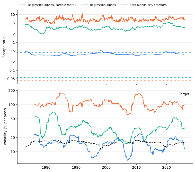
The sign of the market premium
Why fix the premium at 6%? Zero alphas with the trailing 120-month premium do better than the regression alphas but not well, with a Sharpe ratio of 0.24 in Table 1. The problem is the premium’s sign. Figure 2 shows the average market excess return over the previous ten years. It was negative from 1974 to 1979, in 1982, and from 2008 to 2010, and in those months the CAPM investor expects every stock with a positive beta to lose money and shorts all of them.
prem = 100 * col("Trailing premium", "", "value")
fig, ax = plt.subplots(figsize=(8, 3.5))
ax.plot(prem, color="#2a78d6", linewidth=2)
ax.fill_between(prem.index, prem, 0, where=prem < 0, color="#eb6834", alpha=0.4,
                interpolate=True)
ax.axhline(0, color="black", linewidth=0.8)
ax.set_ylabel("Market premium (% per year)")
ax.grid(axis="y", color="#e5e5e5", linewidth=0.8)
ax.spines[["top", "right"]].set_visible(False)
plt.tight_layout()
plt.show()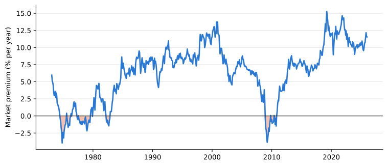
Ten years of data cannot settle the sign of the market premium. Merton (1980) shows why: the precision of an estimated mean depends only on the length of the sample in years, not on the number of observations, so monthly or daily data do not help. Theory settles the sign, though, because investors hold the market only if it pays them for its risk. We fix the premium at 6% per year, although only its sign matters for the zero-alpha means. The CAPM investor then has a Sharpe ratio of 0.43 and holds almost every stock long without any constraint. It does not beat the market’s 0.45, nor should it: with no alphas, the portfolio is the one of the 100 stocks most correlated with the market, and it can do at most as well.
Short-sale constraints and testing
The long-only constraint helps the regression investor the most. It cuts the gross exposure to about one and the holdings to 13 stocks with the sample matrix and 19 with the index-model matrix, and the realized Sharpe ratios rise to 0.50 and 0.41, although the investor still expects three to four and a half times as much. The 0.50, the highest Sharpe ratio in the table, comes from 13 stocks chosen for their average returns over the past ten years, a concentrated bet that past winners keep winning.
Merton (1980)’s point applies to this table as well as to the investor. The second column of Table 1 tests each Sharpe ratio against the market’s, a test that is more precise the more correlated the two portfolios are. The unconstrained portfolios from the regression alphas are worse than the market, with p-values of 0.04 and 0.02. No portfolio is better at any conventional level: the long-only portfolio with 0.50 has a p-value of 0.57, and the CAPM investor’s portfolio, almost perfectly correlated with the market, has 0.71. Half a century of data is enough to show that an optimizer fed regression alphas fails, and not enough to rank the portfolios that do not.
Merton, Robert C. 1980. “On Estimating the Expected Return on the Market: An Exploratory Investigation.” Journal of Financial Economics 8 (4): 323–61.
Shrinking the alphas
Black and Litterman (1992) use equilibrium expected returns, those that make the market portfolio optimal, as a neutral starting point and tilt them toward the investor’s views. The zero-alpha means with a fixed premium play that role here, and the regression alphas play the views. We blend the two, \hat\mu(\lambda) = \lambda\,\hat\beta\,\pi + (1 - \lambda)\,\bar R = (1 - \lambda)\,\hat\alpha + \hat\beta\,\bigl[\lambda\,\pi + (1 - \lambda)\,\bar R_M\bigr], \qquad 0 \leq \lambda \leq 1, with \pi the 6% premium and \bar R the vector of sample means, and form the tangency portfolio with the index-model matrix. The blend shrinks each regression alpha toward zero by the factor 1 - \lambda, and the premium toward 6%. Unlike before, the size of the premium now matters, since it sets how much the prior weighs against the alphas at each \lambda.
Black, Fischer, and Robert Litterman. 1992. “Global Portfolio Optimization.” Financial Analysts Journal 48 (5): 28–43.
blend = pd.DataFrame({c: [stats(("Blend", lam, c))["Sharpe ratio"] for lam in LAMBDAS]
                      for c in ("Unconstrained", "Long-only")}, index=LAMBDAS)
fig, ax = plt.subplots(figsize=(8, 4))
ax.plot(blend.index, blend["Unconstrained"], label="Unconstrained", color="#eb6834",
        linewidth=2, marker="o", markersize=6)
ax.plot(blend.index, blend["Long-only"], label="Long-only", color="#2a78d6",
        linewidth=2, marker="o", markersize=6)
ax.axhline(stats(("CRSP VW", ""))["Sharpe ratio"], color="black", linewidth=1, linestyle="--")
ax.text(0, stats(("CRSP VW", ""))["Sharpe ratio"] + 0.01, "CRSP VW", va="bottom")
ax.set_xlabel(r"Weight $\lambda$ on zero alphas")
ax.set_ylabel("Sharpe ratio")
ax.set_ylim(bottom=0)
ax.grid(axis="y", color="#e5e5e5", linewidth=0.8)
ax.spines[["top", "right"]].set_visible(False)
ax.legend(frameon=False, loc="center left")
plt.tight_layout()
plt.show()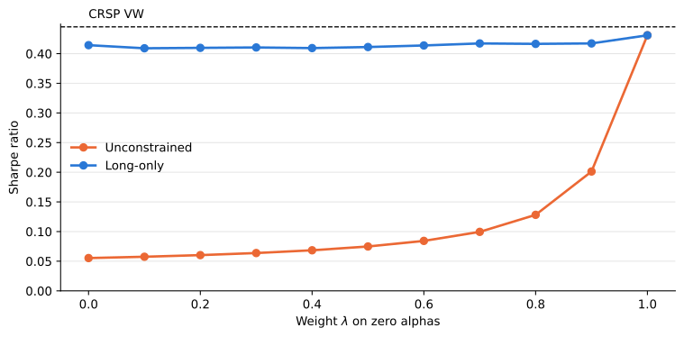
A tenth of the regression alphas is enough to halve the Sharpe ratio. In Figure 3 the unconstrained portfolio has 0.43 at \lambda = 1 and 0.20 at \lambda = 0.9, and up to \lambda = 0.6 it stays between 0.06 and 0.08, no better than the regression alphas alone. The alphas carry nothing that survives out of sample, and a small dose of them spoils the portfolio. The long-only portfolios stay between 0.41 and 0.43 at every \lambda, since the constraint already limits the damage. None of them reaches the market.
What we learned
An investor who runs the index-model regressions and keeps the alphas does not beat the CAPM investor who sets them to zero, and does significantly worse than the market. The regression alphas are the sample means in another form, and their noise is predictable: with 100 stocks and ten years of returns, it is worth a Sharpe ratio of 3.16 to the optimizer, more than any plausible true alpha. In the simulations of Estimation Error in the Tangency Portfolio, the noise falls below the signal only after about 170 years of data, the same order as the 3,000 months that DeMiguel et al. (2009) find the sample tangency portfolio of 25 assets needs to beat 1/N. In the data, the regression investor expects a Sharpe ratio between 2 and 10 every month and earns 0.04 or 0.06. The long-only constraint and shrinkage toward zero alphas limit the damage without beating the market.
DeMiguel, Victor, Lorenzo Garlappi, and Raman Uppal. 2009. “Optimal Versus Naive Diversification: How Inefficient Is the 1/N Portfolio Strategy?” Review of Financial Studies 22 (5): 1915–53.
Ten years of data do not settle even the sign of the market premium, so the CAPM investor takes it from theory and holds the portfolio of the 100 stocks closest to the market, which earns about the market’s Sharpe ratio. An investor whose only information is past returns should index.
The covariance matrix did little here, because the alphas were noise and there was nothing for it to weigh against residual risk. With known alphas, the simulations show the index-model matrix capturing most of the Sharpe ratio available and the sample matrix less than half. A structured covariance matrix pays off for an investor whose alphas come from somewhere other than past returns.