import numpy as np
import pandas as pd
import matplotlib.pyplot as plt
from matplotlib.ticker import FixedLocator, NullLocator, StrMethodFormatter
from threadpoolctl import threadpool_limits
from _portfolio import load_wrds, load_jkp, sharpe, summarize, factor_regression

# Small matrices solve faster on a few threads than on all cores
threadpool_limits(4)

jkp = load_jkp("jkp_usa_all_factors_monthly_vw_cap",
               "https://jkpfactors-data.s3.amazonaws.com/public/"
               "%5Busa%5D_%5Ball_factors%5D_%5Bmonthly%5D_%5Bvw_cap%5D.zip")

ff = load_wrds("ff_factors_monthly_1963_2025", """
    SELECT date, rf
    FROM ff.factors_monthly
    WHERE date BETWEEN '1963-01-01' AND '2025-12-31'
""")

ff5 = load_wrds("ff_fivefactors_monthly_1963_2025", """
    SELECT date, mktrf, smb, hml, rmw, cma, umd
    FROM ff.fivefactors_monthly
    WHERE date BETWEEN '1963-01-01' AND '2025-12-31'
""")

F = jkp.pivot(index="date", columns="name", values="ret")
F.index = F.index.to_period("M")
F = F.loc[F.notna().all(axis=1).idxmax():]
ff6 = ff5.set_index(ff5["date"].dt.to_period("M")).drop(columns="date").astype(float)
rf = ff.set_index(ff["date"].dt.to_period("M"))["rf"].astype(float)

oos = pd.period_range("1992-01", "2025-12", freq="M")An SDF for the Factor Zoo
Computed on October 9, 2026.
The previous notebooks estimated only covariances. The minimum-variance portfolio ignores expected returns, and for good reason: the precision of an estimated mean depends on the length of the sample in calendar time (Merton 1980), so means are much harder to estimate than covariances. Every other mean-variance portfolio needs them. Here we estimate the maximum-Sharpe portfolio of the 153 U.S. factors of Jensen et al. (2023). The same portfolio defines the stochastic discount factor (SDF) that prices those factors (Hansen and Jagannathan 1991), so estimating it amounts to estimating an asset pricing model with 153 factors, a large part of what Cochrane (2011) called the factor zoo.
Merton, Robert C. 1980. “On Estimating the Expected Return on the Market: An Exploratory Investigation.” Journal of Financial Economics 8 (4): 323–61.
Cochrane, John H. 2011. “Presidential Address: Discount Rates.” The Journal of Finance 66 (4): 1047–108.
Hellum, Oliver, Theis I. Jensen, Bryan T. Kelly, and Semyon Malamud. 2026. Complex Modern Portfolio Theory. Working Paper No. 35246. National Bureau of Economic Research.
Two lines of research guide the estimate. Kozak et al. (2020) argue that the SDF needs many factors and that its weights must be shrunk, and they derive a ridge penalty from economic reasoning. The “virtue of complexity” literature argues that models with more parameters than observations can still do well out of sample (Kelly et al. 2024; Didisheim et al. 2023), and Hellum et al. (2026) derive for the GMV portfolio the pattern the previous notebook found in the data. The question is whether that pattern carries over once expected returns enter.
Data
The factors come from the public data of Jensen et al. (2023). Each factor buys the top third of U.S. stocks sorted on one characteristic and sells the bottom third, with value weights capped at the 80th percentile of NYSE market capitalizations so that a few giant firms do not dominate. Each factor is signed so that its long leg is the one the original study found to earn higher returns, which makes most of the 153 average returns positive. All 153 factors have returns from November 1971 on, where our sample starts, to December 2025. The risk-free rate and the six Fama-French factors come from WRDS as before. The market is the Fama-French excess market return rather than the CRSP index, which on WRDS ends in December 2024.
Jensen, Theis Ingerslev, Bryan Kelly, and Lasse Heje Pedersen. 2023. “Is There a Replication Crisis in Finance?” The Journal of Finance 78 (5): 2465–518.
The longest estimation window below is 240 months, so all strategies are evaluated out of sample over the same 408 months, January 1992 to December 2025.
The ridge SDF
Let F_t be the vector of N factor returns in month t. Since each factor is a long-short excess return, an SDF M_t prices all of them if \operatorname{E}[M_t F_t] = 0. With M_t = 1 - w^\top F_t, this condition gives
w = \operatorname{E}[F_t F_t^\top]^{-1} \operatorname{E}[F_t], \tag{1}
and the portfolio w^\top F_t is the maximum-Sharpe portfolio of the factors (Hansen and Jagannathan 1991). Replacing the expectations with sample moments is the same as regressing a constant on the factor returns without an intercept, which gives the sample tangency portfolio (Britten-Jones 1999). Using the second-moment matrix instead of the covariance matrix changes only the scale of w, not its direction.
Hansen, Lars Peter, and Ravi Jagannathan. 1991. “Implications of Security Market Data for Models of Dynamic Economies.” Journal of Political Economy 99 (2): 225–62.
Britten-Jones, Mark. 1999. “The Sampling Error in Estimates of Mean-Variance Efficient Portfolio Weights.” The Journal of Finance 54 (2): 655–71.
The sample version fails for the same reason as the sample GMV portfolio. Write the eigenvalues of the sample second-moment matrix as \lambda_j and its eigenvectors, the principal components of the factors, as v_j. The sample version of (1) puts a weight of v_j^\top \bar F / \lambda_j on each component, where \bar F is the vector of sample means. Components with tiny sample variance get the largest weights, and their sample means are mostly noise. Kozak et al. (2020) argue that an investor should not expect large Sharpe ratios on low-variance components, because arbitrageurs would have competed them away, and show that this prior leads to a ridge penalty. With a penalty z, the weights become
w(z) = \left(\frac{1}{T} \sum_{s} F_s F_s^\top + z \bar{\lambda} I\right)^{-1} \bar{F} = \sum_j \frac{v_j^\top \bar F}{\lambda_j + z \bar\lambda} \, v_j, \tag{2}
where the sum runs over the components with positive sample variance. Here \bar{\lambda} is the average eigenvalue, so z is unit-free. The penalty barely affects components with large variance and strongly shrinks those with small variance. As z grows, the weights become proportional to \bar F, so each factor is weighted by its past average return.
At z = 0 we take the minimum-norm, or ridgeless, solution, which drops the components with zero sample variance. When T > N it is the sample tangency portfolio. When T \leq N the regression of a constant on the factors fits perfectly: the ridgeless portfolio earns exactly the same return in every month of the window, so in sample it looks riskless, like the zero-variance portfolios of the first notebook. Each month we scale the weights to a gross exposure of one, so that the size of the bet does not change from month to month with the estimation noise.
ridge_sdf computes (2) for a grid of penalties from one singular value decomposition of the window’s returns. sdf_returns rolls a window of T months forward and records the next month’s return of each portfolio. select_z chooses a penalty using only information available at the time, as described below.
zs = np.r_[0.0, 10.0 ** np.arange(-4, 1.01, 0.5)]

def ridge_sdf(X, zs):
    T, N = X.shape
    mu = X.mean(axis=0)
    _, s, Vt = np.linalg.svd(X / np.sqrt(T), full_matrices=False)
    lam = s ** 2
    keep = lam > 1e-10 * lam.max()
    lam, Vt = lam[keep], Vt[keep]
    m = Vt @ mu
    scale = (s ** 2).sum() / N
    W = []
    for z in zs:
        if z == 0:
            w = Vt.T @ (m / lam)
        else:
            a = z * scale
            w = Vt.T @ (m / (lam + a)) + (mu - Vt.T @ m) / a
        W.append(w / np.abs(w).sum())
    return np.array(W)

def sdf_returns(F, T, zs, start=None):
    X, idx = F.to_numpy(), F.index
    t0 = T if start is None else max(T, idx.get_loc(pd.Period(start, "M")))
    R = [ridge_sdf(X[t - T:t], zs) @ X[t] for t in range(t0, len(idx))]
    return pd.DataFrame(R, index=idx[t0:], columns=zs)

def select_z(R, burn=60):
    # Each month, the z with the highest Sharpe ratio on past out-of-sample returns
    sr = (R.expanding(burn).mean() / R.expanding(burn).std()).shift(1).dropna(how="all")
    best = sr.idxmax(axis=1)
    return pd.Series([R.at[t, z] for t, z in best.items()], index=best.index), best
Shrinkage
Table 1 and Figure 1 report the out-of-sample Sharpe ratio of the SDF for windows of 12 to 240 months and penalties from zero to 10.
windows = [12, 24, 60, 120, 240]
R = {T: sdf_returns(F, T, zs) for T in windows}
sr_z = pd.DataFrame({T: sharpe(R[T].loc[oos]) for T in windows})
sr_z.index.name = "z"
sr_z.round(2)| 12 | 24 | 60 | 120 | 240 | |
|---|---|---|---|---|---|
| z | |||||
| 0.000000 | 1.02 | 1.09 | 1.01 | 0.64 | 1.05 |
| 0.000100 | 1.02 | 1.09 | 1.02 | 0.69 | 1.08 |
| 0.000316 | 1.02 | 1.09 | 1.03 | 0.77 | 1.12 |
| 0.001000 | 1.02 | 1.09 | 1.06 | 0.93 | 1.22 |
| 0.003162 | 1.02 | 1.10 | 1.14 | 1.17 | 1.37 |
| 0.010000 | 1.02 | 1.11 | 1.27 | 1.39 | 1.56 |
| 0.031623 | 1.02 | 1.14 | 1.42 | 1.57 | 1.74 |
| 0.100000 | 1.03 | 1.19 | 1.57 | 1.73 | 1.88 |
| 0.316228 | 1.02 | 1.23 | 1.67 | 1.86 | 1.97 |
| 1.000000 | 0.98 | 1.18 | 1.62 | 1.86 | 1.93 |
| 3.162278 | 0.86 | 0.96 | 1.39 | 1.69 | 1.73 |
| 10.000000 | 0.66 | 0.62 | 1.00 | 1.36 | 1.41 |
x0 = zs[1] / 10 ** 0.75
xs = np.r_[x0, zs[1:]]
colors = ["#eb6834", "#d4a017", "#2a78d6", "#3a9e5c", "#7a4fb5"]

fig, ax = plt.subplots(figsize=(8, 4.5))
for T, col in zip(windows, colors):
    ax.plot(xs[1:], sr_z[T].iloc[1:], color=col, marker="o", ms=4, label=f"T = {T}, c = {F.shape[1] / T:.2g}")
    ax.scatter([x0], [sr_z[T].iloc[0]], color=col, marker="s", s=40)
ax.axhline(sharpe(F.loc[oos].mean(axis=1)), color="#888888", linestyle=":", linewidth=1)
ax.axhline(sharpe(ff6.loc[oos, "mktrf"]), color="#888888", linestyle=":", linewidth=1)
ax.set_xscale("log")
ax.xaxis.set_major_locator(FixedLocator([x0, 1e-4, 1e-3, 1e-2, 1e-1, 1, 10]))
ax.xaxis.set_minor_locator(NullLocator())
ax.set_xticklabels(["0", "$10^{-4}$", "$10^{-3}$", "$10^{-2}$", "$10^{-1}$", "1", "10"])
ax.set_xlabel("Ridge penalty $z$")
ax.set_ylabel("Sharpe ratio")
ax.grid(axis="y", color="#e5e5e5", linewidth=0.8)
ax.spines[["top", "right"]].set_visible(False)
ax.legend(frameon=False)
plt.tight_layout()
plt.show()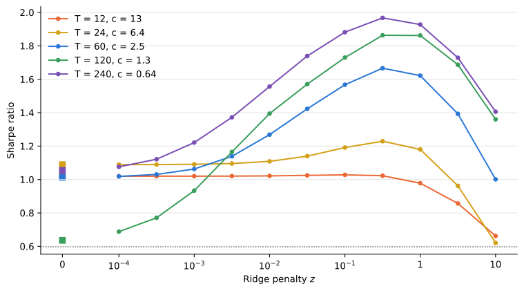
Shrinkage matters most with long windows. With 120 months of data the ridgeless SDF has a Sharpe ratio of 0.64, barely above the market’s, and a penalty of z = 0.32 raises it to 1.86. With 240 months the gain is from 1.05 to 1.97. For every window of 24 months or more the best penalty is z = 0.32, and the Sharpe ratio falls again for larger penalties as the weights approach those of the past average returns.
With 12 months of data the penalty hardly matters until z = 1. The reason is the scaling of the penalty. With T < N there are only T positive eigenvalues, and they share the whole trace, so their average is N / T times \bar\lambda. Relative to these eigenvalues, the effective penalty is z T / N, which at T = 12 is less than a tenth of z. The shorter the window, the larger the penalty that is needed to change anything.
All the shrunk SDFs beat 1/N across factors, which earns 0.60, as does the market. DeMiguel et al. (2009) find the naive 1/N portfolio hard to beat out of sample. Among factors, estimating the means pays off as long as the estimate is shrunk.
DeMiguel, Victor, Lorenzo Garlappi, and Raman Uppal. 2009. “Optimal Versus Naive Diversification: How Inefficient Is the 1/N Portfolio Strategy?” Review of Financial Studies 22 (5): 1915–53.
Complexity
The previous notebook measured complexity as N / (T - 1), the number of assets per direction a demeaned covariance matrix can see. Without demeaning, the second-moment matrix has rank \min(N, T), so here the complexity is c = N / T. We vary c in two ways: the window length T with all 153 factors, and the number of factors N with T = 60, averaging over 10 random subsets of factors for each N.
z_show = [0.0, 0.1]
T_grid = [6, 12, 24, 36, 60, 90, 120, 140, 153, 170, 200, 240]
cT = pd.DataFrame({T: sharpe(sdf_returns(F, T, z_show, start="1992-01")) for T in T_grid}).T
cT["c"] = F.shape[1] / cT.index

rng = np.random.default_rng(0)
N_grid = [6, 12, 24, 36, 48, 60, 72, 96, 120, 153]
cN = {}
for N in N_grid:
    draws = 1 if N == F.shape[1] else 10
    cN[N] = pd.concat([sharpe(sdf_returns(F[rng.choice(F.columns, N, replace=False)], 60, z_show, start="1992-01"))
                       for _ in range(draws)], axis=1).mean(axis=1)
cN = pd.DataFrame(cN).T
cN["c"] = cN.index / 60
fig, ax = plt.subplots(figsize=(8, 4.5))
for z, col in zip(z_show, ("#eb6834", "#2a78d6")):
lab = "Ridgeless" if z == 0 else f"z = {z:g}"
ax.plot(cT["c"], cT[z], color=col, marker="o", ms=5, label=f"{lab}, N = 153")
ax.plot(cN["c"], cN[z], color=col, marker="s", ms=5, linestyle="--", label=f"{lab}, T = 60")
ax.axvline(1, color="#888888", linestyle="--", linewidth=1)
ax.set_xscale("log")
ax.xaxis.set_major_formatter(StrMethodFormatter("{x:g}"))
ax.set_xlabel("Complexity $c = N / T$")
ax.set_ylabel("Sharpe ratio")
ax.grid(axis="y", color="#e5e5e5", linewidth=0.8)
ax.spines[["top", "right"]].set_visible(False)
ax.legend(frameon=False)
plt.tight_layout()
plt.show()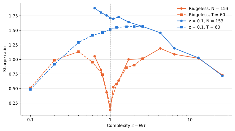
pd.concat({"Vary T, N = 153": cT, "Vary N, T = 60": cN}).round(2)| 0.0 | 0.1 | c | ||
|---|---|---|---|---|
| Vary T, N = 153 | 6 | 0.73 | 0.72 | 25.50 |
| 12 | 1.02 | 1.03 | 12.75 | |
| 24 | 1.09 | 1.19 | 6.38 | |
| 36 | 1.19 | 1.46 | 4.25 | |
| 60 | 1.01 | 1.57 | 2.55 | |
| 90 | 1.00 | 1.64 | 1.70 | |
| 120 | 0.64 | 1.73 | 1.27 | |
| 140 | 0.52 | 1.70 | 1.09 | |
| 153 | 0.13 | 1.71 | 1.00 | |
| 170 | 0.44 | 1.76 | 0.90 | |
| 200 | 0.82 | 1.81 | 0.76 | |
| 240 | 1.05 | 1.88 | 0.64 | |
| Vary N, T = 60 | 6 | 0.51 | 0.49 | 0.10 |
| 12 | 0.99 | 0.92 | 0.20 | |
| 24 | 1.13 | 1.29 | 0.40 | |
| 36 | 0.95 | 1.41 | 0.60 | |
| 48 | 0.74 | 1.46 | 0.80 | |
| 60 | 0.21 | 1.52 | 1.00 | |
| 72 | 0.58 | 1.55 | 1.20 | |
| 96 | 0.86 | 1.56 | 1.60 | |
| 120 | 0.90 | 1.57 | 2.00 | |
| 153 | 1.01 | 1.57 | 2.55 |
The ridgeless SDF repeats the pattern of the GMV portfolio. Its Sharpe ratio falls to 0.13 at c = 1 when we vary T, and to 0.21 when we vary N. The two curves have different factors and windows but nearly the same shape, so here too c rather than N or T alone governs the damage. Near c = 1 the smallest positive eigenvalues approach zero, and (2) puts huge weights on noise. Past c = 1 the Sharpe ratio recovers, to 1.19 at c = 4.25 and 1.02 at c = 12.75, a model with 153 parameters estimated from 12 months of data. This is the double descent of ridgeless regression (Hastie et al. 2022), which Kelly et al. (2024) and Didisheim et al. (2023) call the virtue of complexity.
Hastie, Trevor, Andrea Montanari, Saharon Rosset, and Ryan J. Tibshirani. 2022. “Surprises in High-Dimensional Ridgeless Least Squares Interpolation.” The Annals of Statistics 50 (2): 949–86.
Kelly, Bryan, Semyon Malamud, and Kangying Zhou. 2024. “The Virtue of Complexity in Return Prediction.” The Journal of Finance 79 (1): 459–503.
Didisheim, Antoine, Shikun Barry Ke, Bryan T. Kelly, and Semyon Malamud. 2023. Complexity in Factor Pricing Models. Working Paper No. 31689. National Bureau of Economic Research.
A penalty of z = 0.1 removes the dip. With all 153 factors, the Sharpe ratio rises almost steadily with the window, from 0.72 at T = 6 to 1.88 at T = 240, so more data help once the estimate is shrunk. With T = 60, adding factors raises it from 0.49 with 6 factors to 1.52 with 60 and 1.57 with 120 or more. Additional factors never hurt the shrunk SDF, and they still help a little past c = 1. This is the sense of the finding of Didisheim et al. (2023) that the best SDF has more factors than observations.
Unlike in the GMV case, high complexity does not match low complexity here. The best ridgeless SDF at c > 1 has a Sharpe ratio of 1.19, against 1.88 for the shrunk SDF with 240 months. Expected returns are estimated much less precisely than covariances, so the estimate needs both a long sample and shrinkage. Complexity alone does not substitute for data.
Performance
The best penalty in Table 1 is known only after the fact. An investor has to choose it with past data. Each month, select_z computes the Sharpe ratio that each penalty would have delivered out of sample up to the previous month and picks the highest, after a burn-in of 60 months. The windows of 60 and 120 months start early enough for this history to be available by 1992.
We compare the result with three benchmarks: the market, 1/N across the 153 factors, and FF6, the tangency portfolio of the five Fama-French factors (Fama and French 2015) and momentum (Carhart 1997), estimated the same way with 120 months. Each strategy is scaled after the fact to the market’s volatility over 1992 to 2025. Scaling does not change Sharpe ratios, betas, t-statistics or R^2, and it puts means and drawdowns on a common footing.
Fama, Eugene F., and Kenneth R. French. 2015. “A Five-Factor Asset Pricing Model.” Journal of Financial Economics 116 (1): 1–22.
Carhart, Mark M. 1997. “On Persistence in Mutual Fund Performance.” Journal of Finance 52 (1): 57–82.
fmt = lambda x: "" if pd.isna(x) else f"{round(x, 2) + 0.0:.2f}"
cv = {T: select_z(R[T]) for T in (60, 120)}

strategies = {
    "1/N": F.loc[oos].mean(axis=1),
    "FF6, T = 120": sdf_returns(ff6, 120, [0.0])[0.0],
    "Ridgeless, T = 12": R[12][0.0],
    "Ridgeless, T = 120": R[120][0.0],
    "Ridge CV, T = 60": cv[60][0],
    "Ridge CV, T = 120": cv[120][0],
}
mkt_ex, rf_o = ff6.loc[oos, "mktrf"], rf.loc[oos]
vol = mkt_ex.std()

def stats(ex):
    ex = ex.loc[oos] * vol / ex.loc[oos].std()
    coef, p, r2 = factor_regression(ex + rf_o, rf_o, ff6.loc[oos])
    return pd.concat([summarize(ex + rf_o, mkt_ex + rf_o, rf_o),
                      pd.Series({"FF6 alpha (%)": 1200 * coef[0], "FF6 alpha p-value": p[0], "FF6 R2": r2})])

tbl = pd.DataFrame({name: stats(ex) for name, ex in strategies.items()})
tbl.insert(0, "Market", summarize(mkt_ex + rf_o, mkt_ex + rf_o, rf_o))
tbl.map(fmt)| Market | 1/N | FF6, T = 120 | Ridgeless, T = 12 | Ridgeless, T = 120 | Ridge CV, T = 60 | Ridge CV, T = 120 | |
|---|---|---|---|---|---|---|---|
| Mean (%) | 11.44 | 11.42 | 16.40 | 17.80 | 12.02 | 27.45 | 29.84 |
| Volatility (%) | 15.05 | 15.10 | 15.08 | 15.14 | 15.11 | 15.22 | 15.18 |
| Sharpe ratio | 0.60 | 0.60 | 0.93 | 1.02 | 0.64 | 1.66 | 1.82 |
| Beta | 1.00 | -0.57 | 0.33 | -0.20 | 0.02 | -0.06 | -0.11 |
| Alpha (%) | 0.00 | 14.05 | 10.98 | 17.12 | 9.43 | 25.55 | 28.38 |
| Alpha p-value | 0.00 | 0.00 | 0.00 | 0.00 | 0.00 | 0.00 | |
| Max drawdown (%) | -50.31 | -41.91 | -26.54 | -24.76 | -44.68 | -16.42 | -18.44 |
| FF6 alpha (%) | 5.65 | 0.11 | 12.42 | 7.45 | 21.68 | 23.96 | |
| FF6 alpha p-value | 0.00 | 0.94 | 0.00 | 0.01 | 0.00 | 0.00 | |
| FF6 R2 | 0.86 | 0.67 | 0.21 | 0.06 | 0.11 | 0.12 |
Choosing the penalty with past data costs little. The SDF with 120 months has a Sharpe ratio of 1.82, against 1.86 with the best penalty chosen after the fact, and with 60 months the figures are 1.66 and 1.67. Figure 3 shows that the selection moves between three neighboring values and settles at z = 0.32, the best value after the fact, for most of the period after 2005.
The shrunk SDFs reach about three times the market’s Sharpe ratio and twice that of FF6, with maximum drawdowns of 16% to 18% against 50% for the market. Their market betas are close to zero. Regressed on the six Fama-French factors, they have alphas of 22% to 24% a year at the market’s volatility and an R^2 of about 0.12, so they are mostly unrelated to the usual factors. The ridgeless SDF with 120 months, at c = 1.3, near the peak of Figure 2, does no better than the market. FF6 has a Sharpe ratio of 0.93 but no alpha on its own factors, as expected. The 1/N portfolio has a negative market beta of -0.57: many anomalies buy low-risk stocks and sell high-risk ones, so averaging the signed factors gives a short position in the market.
These are returns on paper. They ignore trading costs, which matter because the factors trade small and illiquid stocks, rebalance often, and the SDF combines them with long and short positions. The means near 30% a year are not attainable at that volatility.
Subperiods
Figure 4 suggests that most of the growth of the shrunk SDFs happened before about 2005. Factors are known to lose part of their returns after the study that documents them is published: McLean and Pontiff (2016) find average returns 58% lower after publication across 97 predictors. There is also a selection effect. The 153 factors are those that researchers had found and published by the time the data set was assembled, and many were discovered with data that overlap our sample. An investor in 1992 could not have traded most of them. With hundreds of characteristics tested, some must look significant by chance (Harvey et al. 2016), and those factors should not earn their in-sample returns afterward. If the SDF earns its Sharpe ratio from such factors, it should weaken in later subperiods.
McLean, R. David, and Jeffrey Pontiff. 2016. “Does Academic Research Destroy Stock Return Predictability?” The Journal of Finance 71 (1): 5–32.
Harvey, Campbell R., Yan Liu, and Heqing Zhu. 2016“... And the Cross-Section of Expected Returns.” The Review of Financial Studies 29 (1): 5–68.
periods = {"1992-2004": ("1992-01", "2004-12"), "2005-2014": ("2005-01", "2014-12"),
           "2015-2025": ("2015-01", "2025-12"), "1992-2025": ("1992-01", "2025-12")}
sub = pd.DataFrame({p: {name: sharpe(ex.loc[a:b]) for name, ex in {"Market": mkt_ex, **strategies}.items()}
                    for p, (a, b) in periods.items()})
sub.map(fmt)| 1992-2004 | 2005-2014 | 2015-2025 | 1992-2025 | |
|---|---|---|---|---|
| Market | 0.52 | 0.50 | 0.76 | 0.60 |
| 1/N | 0.76 | 0.70 | 0.36 | 0.60 |
| FF6, T = 120 | 1.26 | 0.79 | 0.73 | 0.93 |
| Ridgeless, T = 12 | 1.65 | 0.56 | 0.69 | 1.02 |
| Ridgeless, T = 120 | 1.09 | 0.13 | 0.43 | 0.64 |
| Ridge CV, T = 60 | 2.74 | 1.09 | 0.76 | 1.66 |
| Ridge CV, T = 120 | 2.87 | 1.26 | 1.04 | 1.82 |
Table 4 confirms the decline. From 1992 to 2004 the shrunk SDFs have Sharpe ratios of 2.74 and 2.87. From 2005 to 2014 these fall to 1.09 and 1.26, and from 2015 to 2025 to 0.76 and 1.04. The 1/N portfolio falls from 0.76 to 0.36, and FF6 from 1.26 to about 0.75, while the market’s Sharpe ratio rises from 0.52 to 0.76. Over the last decade only the shrunk SDF with 120 months clearly beats the market.
The decline is not only a matter of estimation. Every factor strategy falls, including 1/N, which estimates nothing, and the best-regularized SDF loses as much as the ridgeless ones. The factors themselves earn less than before.
fig, ax = plt.subplots(figsize=(8, 3))
levels = np.unique(np.r_[cv[60][1].loc[oos], cv[120][1].loc[oos]])
for T, col in zip((60, 120), ("#2a78d6", "#3a9e5c")):
    z = cv[T][1].loc[oos]
    ax.step(z.index.to_timestamp(), z.where(z > 0, x0), where="post", color=col, label=f"T = {T}")
ax.set_yscale("log")
ax.yaxis.set_major_locator(FixedLocator(np.where(levels > 0, levels, x0)))
ax.yaxis.set_minor_locator(NullLocator())
ax.set_yticklabels([f"{z:.2g}" for z in levels])
ax.set_ylabel("Selected $z$")
ax.grid(axis="y", color="#e5e5e5", linewidth=0.8)
ax.spines[["top", "right"]].set_visible(False)
ax.legend(frameon=False)
plt.tight_layout()
plt.show()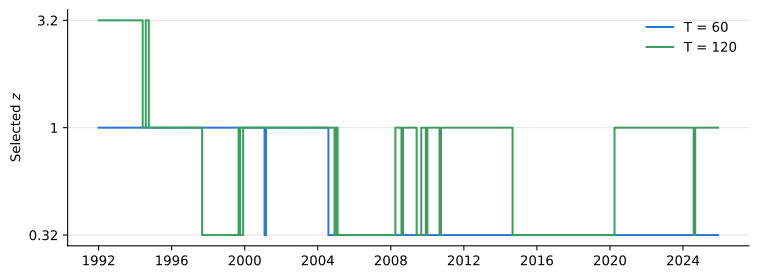
fig, ax = plt.subplots(figsize=(8, 4.5))
series = {"Market": mkt_ex, **{k: v.loc[oos] * vol / v.loc[oos].std() for k, v in strategies.items()}}
for (name, ex), col in zip(series.items(), ["#888888", "#b0b0b0", "#7a4fb5", "#eb6834", "#d4a017", "#2a78d6", "#3a9e5c"]):
    ax.plot(ex.index.to_timestamp(), (1 + ex).cumprod(), color=col, linewidth=1.2, label=name)
ax.set_yscale("log")
ax.yaxis.set_major_formatter(StrMethodFormatter("{x:g}"))
ax.set_ylabel(r"Growth of \$1")
ax.grid(axis="y", color="#e5e5e5", linewidth=0.8)
ax.spines[["top", "right"]].set_visible(False)
ax.legend(frameon=False)
plt.tight_layout()
plt.show()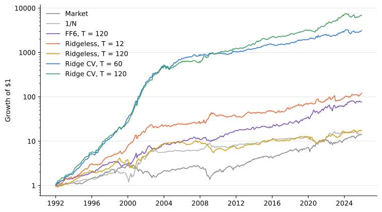
What we learned
The SDF of the factor zoo behaves like the GMV portfolio with respect to complexity. The ridgeless estimate breaks down near c = 1 and recovers on either side, and a ridge penalty removes the breakdown. Unlike the GMV portfolio, the SDF depends on expected returns, which are estimated imprecisely, so a long window and shrinkage are both needed. With 120 to 240 months of data and a penalty around z = 0.32, the SDF of 153 factors has an out-of-sample Sharpe ratio near 1.9, and choosing the penalty from past data gives up little of that.
The ridge penalty of Kozak et al. (2020) shrinks every component by the same amount relative to its variance. Kelly et al. (2023) propose a shrinkage function estimated from the data that reweights the components more flexibly, which is a natural next step. The larger caveat is time. Most of the SDF’s performance comes before 2005, and since then its Sharpe ratio has been closer to that of the market. Whether the decline reflects publication, selection of the factors, or both is a question the publication dates in the factor data can help answer.
Kozak, Serhiy, Stefan Nagel, and Shrihari Santosh. 2020. “Shrinking the Cross-Section.” Journal of Financial Economics 135 (2): 271–92.
Kelly, Bryan T., Semyon Malamud, Mohammad Pourmohammadi, and Fabio Trojani. 2023. Universal Portfolio Shrinkage. Working Paper No. 32004. National Bureau of Economic Research.