import contextlib
import io
from pathlib import Path

import numpy as np
import pandas as pd
import matplotlib.pyplot as plt
from threadpoolctl import threadpool_limits

# Small matrices solve faster on one thread than on all cores
threadpool_limits(1)

DATA_DIR = Path("../_data")


def load_wrds(name, sql):
    file = DATA_DIR / f"{name}.parquet"
    if not file.exists():
        import wrds
        with contextlib.redirect_stdout(io.StringIO()):
            conn = wrds.Connection()
        df = conn.raw_sql(sql, date_cols=["date"])
        conn.close()
        DATA_DIR.mkdir(exist_ok=True)
        df.to_parquet(file)
    return pd.read_parquet(file)


crsp_m = load_wrds("crsp_msf_1963_2025", """
    SELECT permno, mthcaldt AS date, mthret AS ret, shrout, mthprc AS prc, mthcap
    FROM crsp.msf_v2
    WHERE mthcaldt BETWEEN '1963-01-01' AND '2025-12-31'
      AND sharetype = 'NS' AND securitytype = 'EQTY'
      AND securitysubtype = 'COM' AND usincflg = 'Y'
      AND issuertype IN ('ACOR', 'CORP')
      AND primaryexch IN ('N', 'A', 'Q')
      AND conditionaltype IN ('RW', 'NW')
""")

crsp_vw = load_wrds("crsp_msi_1963_2025", """
    SELECT mthcaldt AS date, mthtotret AS vwretd
    FROM crsp.indmthseriesdata
    WHERE indno = 1000200
      AND mthcaldt BETWEEN '1963-01-01' AND '2025-12-31'
""")

ff = load_wrds("ff_factors_monthly_1963_2025", """
    SELECT date, rf
    FROM ff.factors_monthly
    WHERE date BETWEEN '1963-01-01' AND '2025-12-31'
""")

crsp_m["mcap"] = crsp_m["prc"].abs() * crsp_m["shrout"] / 1e6
rets = crsp_m.pivot(index="date", columns="permno", values="ret").sort_index().astype(float)
mcaps = crsp_m.pivot(index="date", columns="permno", values="mcap").reindex(rets.index).astype(float)
dates = rets.index
mkt = crsp_vw.set_index("date")["vwretd"].astype(float).reindex(dates)
# Fama-French dates months by their first day and CRSP by the last trading day
rf = pd.Series(ff.set_index(ff["date"].dt.to_period("M"))["rf"].astype(float)
               .reindex(dates.to_period("M")).to_numpy(), index=dates)

WINDOW, TOP_N = 120, 100
t_end = len(dates) - 1
ok = mcaps.iloc[t_end].where(rets.iloc[t_end - WINDOW + 1:].notna().all()).dropna()
ids = ok.nlargest(TOP_N).index
X_cal = rets[ids].sub(rf, axis=0).iloc[t_end - WINDOW + 1:].to_numpy()
m_cal = (mkt - rf).iloc[t_end - WINDOW + 1:].to_numpy()Estimation Error in the Tangency Portfolio
The tangency portfolio, the portfolio of risky assets with the highest Sharpe ratio, has weights proportional to \Sigma^{-1}\mu, where \mu is the vector of expected excess returns and \Sigma the covariance matrix. An investor has to estimate both, and the errors in each do different damage. This notebook separates them with two simulations calibrated to the 100 largest U.S. stocks.
In the first, the investor knows the expected returns, alphas included, and estimates only the covariance matrix. The sample matrix captures less than half of the Sharpe ratio available, while the index model, although it misses the comovement of residual returns, captures most of it. A structured covariance matrix is worth having when the investor has information about expected returns. In the second, the investor estimates the means too, with the regressions of the index model. The noise in the estimated alphas then dominates everything else, by an amount that can be computed before seeing any data. Can Regression Alphas Beat the CAPM? runs the second experiment on 53 years of data.
Calibrating to the 100 largest stocks
Both simulations start from the 100 largest common stocks at the end of 2025 with a return in each of the previous 120 months. The returns are monthly, from crsp.msf_v2, with the CRSP value-weighted index as the market and the one-month T-bill rate from ff, all in excess of the T-bill rate. Each table is saved as a parquet file in _data on the first run. Delete a file to pull it again.
The single index model writes each stock’s excess return as R_i = \alpha_i + \beta_i R_M + e_i. Regressions of each stock on the market give the betas, the residuals and the market variance, which index_model returns. The investor’s index-model matrix is
\hat\Sigma_{\text{IM}} = \hat\sigma_M^2\,\hat\beta\hat\beta^\top + \hat D,
with \hat D the diagonal matrix of residual variances, which treats the residuals as uncorrelated across stocks.
def index_model(X, m):
    """Betas, residuals and market variance from regressions of the columns
    of X on m, with an intercept."""
    mc = m - m.mean()
    Xc = X - X.mean(axis=0)
    b = Xc.T @ mc / (mc @ mc)
    return b, Xc - np.outer(mc, b), m.var(ddof=1)


def sr(w, mu, S):
    """Annualized Sharpe ratio of weights w under means mu and matrix S."""
    return np.sqrt(12) * (w @ mu) / np.sqrt(w @ S @ w)
Known alphas, estimated covariances
In this experiment the truth has more structure than the index model. Residual returns are correlated, as they are among stocks in the same industry, and some of that comovement carries alpha, as characteristics such as value or profitability do relative to the CAPM. The true model adds K = 5 residual factors to the market, R_i = \alpha_i + \beta_i R_M + \sum_{k=1}^{K} b_{ik} f_k + e_i, \qquad \alpha_i = \sum_{k=1}^{K} b_{ik}\,\gamma_k, where the factors f_k have mean zero, unit variance and are uncorrelated with the market and with each other, and \gamma_k is the premium the investor earns for bearing them. The loadings b_{ik} are the first five principal components of the residual covariance matrix of the calibration sample, as in Fan et al. (2013), which leaves the rest of the residual variance as uncorrelated firm-specific risk. Each residual factor has a Sharpe ratio of 0.3 per year, and the market premium is 6% per year. The alphas exist only because of the factors, so a portfolio that bets on them bears factor risk that the index model does not see.
Fan, Jianqing, Yuan Liao, and Martina Mincheva. 2013. “Large Covariance Estimation by Thresholding Principal Orthogonal Complements.” Journal of the Royal Statistical Society: Series B (Statistical Methodology) 75 (4): 603–80.
K, SR_FACTOR, PREMIUM = 5, 0.30, 0.06 / 12

b0, E0, s2m0 = index_model(X_cal, m_cal)
S_e = np.cov(E0, rowvar=False)
eigval, eigvec = np.linalg.eigh(S_e)
eigval, eigvec = eigval[::-1][:K], eigvec[:, ::-1][:, :K]
B0 = eigvec * np.sqrt(eigval)                   # loadings on unit-variance factors
d0 = np.clip(np.diag(S_e) - (B0**2).sum(axis=1), 1e-6, None)
gamma = np.full(K, SR_FACTOR / np.sqrt(12))     # monthly premium per unit of factor risk

mu_true = b0 * PREMIUM + B0 @ gamma
Sig_true = s2m0 * np.outer(b0, b0) + B0 @ B0.T + np.diag(d0)
sr_max = sr(np.linalg.solve(Sig_true, mu_true), mu_true, Sig_true)
sr_mkt = np.sqrt(12) * PREMIUM / np.sqrt(s2m0)
share_k = eigval.sum() / np.trace(S_e)
pd.Series({"Market Sharpe ratio": sr_mkt, "Best attainable Sharpe ratio": sr_max,
           "Residual variance explained by the factors (%)": 100 * share_k}).round(2)
Market Sharpe ratio 0.39
Best attainable Sharpe ratio 0.75
Residual variance explained by the factors (%) 36.00
dtype: float64The alphas nearly double the Sharpe ratio available, from the market’s to the best attainable. Each simulated sample draws 120 months of normal returns from the true model, independent across months, and the investor, who knows \mu, holds the tangency portfolio \hat\Sigma^{-1}\mu for one of three estimates of \Sigma: the sample matrix, the index-model matrix, and a five-factor matrix that adds the first five principal components of the sample’s residuals to the index model. The five-factor investor knows how many factors there are but not what they are.
def estimated_matrices(Y, m, k=K):
    """Sample, index-model and index-plus-k-factor covariance matrices."""
    b, E, s2m = index_model(Y, m)
    S_e = np.cov(E, rowvar=False)
    lam, v = np.linalg.eigh(S_e)
    Bk = v[:, ::-1][:, :k] * np.sqrt(lam[::-1][:k])
    dk = np.clip(np.diag(S_e) - (Bk**2).sum(axis=1), 1e-8, None)
    return b, {"Sample": np.cov(Y, rowvar=False),
               "Index model": s2m * np.outer(b, b) + np.diag(E.var(axis=0, ddof=2)),
               "Five-factor": s2m * np.outer(b, b) + Bk @ Bk.T + np.diag(dk)}


def draw(T, rng):
    """T months of market and stock excess returns from the true model."""
    m = PREMIUM + np.sqrt(s2m0) * rng.standard_normal(T)
    f = gamma + rng.standard_normal((T, K))
    Y = np.outer(m, b0) + f @ B0.T + rng.standard_normal((T, TOP_N)) * np.sqrt(d0)
    return Y, m


rng = np.random.default_rng(1)
rows = []
for _ in range(500):
    Y, m = draw(WINDOW, rng)
    _, mats = estimated_matrices(Y, m)
    row = {}
    for name, S in mats.items():
        w = np.linalg.solve(S, mu_true)
        row[(name, "Investor's estimate")] = sr(w, mu_true, S)
        row[(name, "True value")] = sr(w, mu_true, Sig_true)
    rows.append(row)
known = pd.DataFrame(rows)
known.columns = pd.MultiIndex.from_tuples(known.columns)
tbl_known = known.mean().unstack()
tbl_known["Share of the best (%)"] = 100 * tbl_known["True value"] / sr_max
tbl_known.index.name = "Covariance matrix"
tbl_known.loc[["Sample", "Index model", "Five-factor"]].round(2)| Investor's estimate | True value | Share of the best (%) | |
|---|---|---|---|
| Covariance matrix | |||
| Sample | 1.94 | 0.31 | 41.30 |
| Index model | 1.88 | 0.64 | 85.95 |
| Five-factor | 1.05 | 0.65 | 87.17 |
The sample matrix captures less than half of the Sharpe ratio available, and the index model 86% of it, although it ignores the residual factors that carry every alpha. With 100 stocks and 120 months, the sample matrix has to estimate 5,050 variances and covariances from 12,000 returns, and its inverse understates risk in exactly the directions the optimizer chooses. The index model estimates 201 parameters, and its error is a bias, not noise. Bias wins here: a wrong but stable model beats an unbiased but noisy one.
The bias shows in the investor’s estimates. With the index-model matrix, the investor treats the residual factors as diversifiable firm-specific risk and expects a Sharpe ratio nearly three times the true one. The five-factor matrix sees the factors and corrects most of that error, but it adds only about one percentage point to the share of the best captured. The factors matter for how much risk the investor thinks the portfolio has, much less for the portfolio itself, and most of the value of a structured matrix comes from imposing any structure at all.
Estimated alphas
In the second experiment, the investor estimates the means as well. The index-model regressions give each stock an alpha, and since the intercept satisfies \hat\alpha_i = \bar R_i - \hat\beta_i \bar R_M, the investor who keeps the estimated alphas uses expected returns \hat\mu_i = \hat\alpha_i + \hat\beta_i \bar R_M = \bar R_i, the sample means. The investor who sets every alpha to zero, as the CAPM says, uses \hat\mu_i = \hat\beta_i \bar R_M, and the tangency portfolio is then \hat D^{-1}\hat\beta, the portfolio of the 100 stocks most correlated with the market. To isolate the noise in the means, the truth in this experiment is the index model with no alphas, fitted to the calibration sample, with the market premium at its sample average. Both the means and the matrix are estimated from each simulated sample.
# True parameters: the index model with no alphas, fitted to the calibration sample
d_im = E0.var(axis=0, ddof=2)
pm0, sm0 = m_cal.mean(), np.sqrt(s2m0)
mu0 = b0 * pm0
Sig0 = s2m0 * np.outer(b0, b0) + np.diag(d_im)
sr_best = sr(np.linalg.solve(Sig0, mu0), mu0, Sig0)

SIM_RULES = {
    "Regression alphas | Sample": ("alphas", "Sample"),
    "Regression alphas | Index model": ("alphas", "Index model"),
    "Zero alphas | Index model": ("zero", "Index model"),
}


def simulate(T, n_sims, seed=1):
    rng = np.random.default_rng(seed)
    rows = []
    for _ in range(n_sims):
        m = pm0 + sm0 * rng.standard_normal(T)
        Y = np.outer(m, b0) + rng.standard_normal((T, TOP_N)) * np.sqrt(d_im)
        b, E, s2m = index_model(Y, m)
        mats = {"Sample": np.cov(Y, rowvar=False),
                "Index model": s2m * np.outer(b, b) + np.diag(E.var(axis=0, ddof=2))}
        means = {"alphas": Y.mean(axis=0), "zero": b * m.mean()}
        row = {}
        for name, (mn, sn) in SIM_RULES.items():
            mu_hat, S_hat = means[mn], mats[sn]
            w = np.linalg.solve(S_hat, mu_hat)
            row[(name, "Investor's estimate")] = sr(w, mu_hat, S_hat)
            row[(name, "True value")] = sr(w, mu0, Sig0)
        rows.append(row)
    out = pd.DataFrame(rows)
    out.columns = pd.MultiIndex.from_tuples(out.columns)
    return out


sim120 = simulate(WINDOW, 500)
tbl = sim120.mean().unstack()[["Investor's estimate", "True value"]].reindex(SIM_RULES)
tbl.index = pd.MultiIndex.from_tuples([tuple(k.split(" | ")) for k in tbl.index],
names=["Means", "Covariance matrix"])
tbl.loc[("Best attainable", ""), :] = [np.nan, sr_best]
tbl.map(lambda x: "" if pd.isna(x) else f"{x:.2f}")| Investor's estimate | True value | ||
|---|---|---|---|
| Means | Covariance matrix | ||
| Regression alphas | Sample | 8.32 | 0.07 |
| Index model | 3.37 | 0.28 | |
| Zero alphas | Index model | 0.75 | 0.75 |
| Best attainable | 0.76 |
The investor who sets the alphas to zero does almost as well as possible, as the truth guarantees here. The investor who keeps the estimated alphas does far worse. With the sample matrix, that investor expects a Sharpe ratio above 8 and gets almost nothing, and with the index-model matrix expects above 3 and gets about a third of the best. Ten years of returns say little about a stock’s mean: for a stock with a volatility of 30% per year, the standard error of its average annual return over ten years is 30\%/\sqrt{10}, about 9.5 percentage points, larger than any plausible alpha. The optimizer treats that noise as alpha.
The size of the investor’s error can be predicted before looking at any sample. With sample means and the sample matrix, the investor’s squared Sharpe ratio is \hat\theta^2 = \bar R^\top \hat\Sigma^{-1} \bar R, and with normal returns Kan and Zhou (2007) show that its expected value is E[\hat\theta^2] = \frac{T\theta^2 + N}{T - N - 2} = \frac{T}{T - N - 2}\left(\theta^2 + \frac{N}{T}\right), where \theta^2 = \mu^\top\Sigma^{-1}\mu is the true squared Sharpe ratio per month and \hat\Sigma divides by T. Two sources of overconfidence multiply. The term N/T comes from the means: each sample mean misses its true value by noise with covariance matrix \Sigma/T, so even with the true matrix E[\bar R^\top \Sigma^{-1} \bar R] = \theta^2 + N/T. The factor T/(T - N - 2) comes from inverting the sample matrix. The index-model matrix is close to the true one, so with it the investor’s estimate should be close to \theta^2 + N/T.
Kan, Raymond, and Guofu Zhou. 2007. “Optimal Portfolio Choice with Parameter Uncertainty.” Journal of Financial and Quantitative Analysis 42 (3): 621–56.
theta2 = (sr_best / np.sqrt(12)) ** 2
N, T = TOP_N, WINDOW
pred = {
    # Kan and Zhou divide the sample matrix by T, np.cov by T - 1
    "Sample": (T - 1) / T * (T * theta2 + N) / (T - N - 2),
    "Index model": theta2 + N / T,
}
delusion = pd.DataFrame({
    "Noise in the means": {k: np.sqrt(12 * N / T) for k in pred},
    "Predicted": {k: np.sqrt(12 * v) for k, v in pred.items()},
    "Simulated": {k: np.sqrt((sim120[(f"Regression alphas | {k}", "Investor's estimate")] ** 2).mean())
                  for k in pred},
})
delusion.index.name = "Covariance matrix"
delusion.map(lambda x: f"{x:.2f}")| Noise in the means | Predicted | Simulated | |
|---|---|---|---|
| Covariance matrix | |||
| Sample | 3.16 | 8.36 | 8.46 |
| Index model | 3.16 | 3.25 | 3.38 |
Kan, Raymond, and Guofu Zhou. 2007. “Optimal Portfolio Choice with Parameter Uncertainty.” Journal of Financial and Quantitative Analysis 42 (3): 621–56.
The prediction needs only N, T and the true Sharpe ratio, and the true Sharpe ratio hardly matters: the noise in the means alone is worth a Sharpe ratio of \sqrt{12 N/T} = 3.16, and inverting the sample matrix multiplies the squared Sharpe ratio by another T/(T - N - 2) = 6.7. The noise falls only as N/T, and for it to drop below the signal \theta^2 the sample must be longer than N/\theta^2 months, about 2,000 months or 170 years with the best attainable Sharpe ratio of Table 2. Figure 1 repeats the experiment for samples of 120 to 960 months, 200 samples each.
T_grid = [120, 240, 480, 960]
sweep = pd.DataFrame({T: simulate(T, 200, seed=2).xs("True value", axis=1, level=1).mean()
                      for T in T_grid}).T
from matplotlib.ticker import NullLocator, StrMethodFormatter
fig, ax = plt.subplots(figsize=(8, 4))
series = [("Zero alphas | Index model", "Zero alphas, index-model matrix", "#2a78d6"),
("Regression alphas | Index model", "Regression alphas, index-model matrix", "#1baf7a"),
("Regression alphas | Sample", "Regression alphas, sample matrix", "#eb6834")]
for col, label, color in series:
ax.plot(sweep.index, sweep[col], label=label, color=color,
linewidth=2, marker="o", markersize=6)
ax.axhline(sr_best, color="black", linewidth=1, linestyle="--")
ax.text(T_grid[0], sr_best + 0.02, "Best attainable", va="bottom")
ax.set_xscale("log")
ax.set_xticks(T_grid)
ax.xaxis.set_major_formatter(StrMethodFormatter("{x:g}"))
ax.xaxis.set_minor_locator(NullLocator())
ax.set_xlabel("Months of data $T$")
ax.set_ylabel("True Sharpe ratio")
ax.set_ylim(bottom=0)
ax.grid(axis="y", color="#e5e5e5", linewidth=0.8)
ax.spines[["top", "right"]].set_visible(False)
ax.legend(frameon=False, loc="lower right")
plt.tight_layout()
plt.show()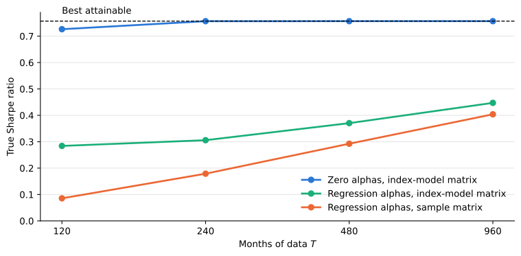
Even 80 years of data leave the estimated alphas far from the best attainable Sharpe ratio. In Table 2 the zero-alpha investor’s success is built in, since the truth has no alphas. The prediction of Table 3 is not: the noise in the estimated alphas is the same whether or not true alphas exist, and only large true alphas could stand out against it.
What we learned
The two inputs of the tangency portfolio fail in different ways. Errors in the covariance matrix are a problem of dimension, and structure solves it: with known expected returns, the index model captures most of the Sharpe ratio available even when its assumption of uncorrelated residuals is wrong, while the sample matrix captures less than half. Errors in the means are a problem of signal to noise, and no structure on the covariance matrix solves it. With 100 stocks and ten years of data, the estimated alphas look to the optimizer like a Sharpe ratio of 3.16, and the sample would have to be about 170 years long before the true expected returns could stand out. A structured covariance matrix pays off for an investor whose information about alphas comes from somewhere other than past returns.