The Index Model

Introduction

One of the disadvantages of the Markowitz model is that it requires estimates of all covariances and expected returns. Estimating the covariance between two assets is not hard, and can be done with precision. The difficulty is their number. For five hundred stocks we would have to estimate 500 \times 501 / 2 = 125{,}250 different variances and covariances, while ten years of monthly data provide only 500 \times 120 = 60{,}000 returns. When the stocks outnumber the months, the sample covariance matrix is singular: some portfolios appear to have no risk at all, which is an artifact of the sample. With fewer stocks the matrix can be inverted, but the noise does not go away. It is largest in the portfolios that look least risky, which are exactly the ones an optimizer loads on (Laloux et al. 1999).

Laloux, Laurent, Pierre Cizeau, Jean-Philippe Bouchaud, and Marc Potters. 1999. “Noise Dressing of Financial Correlation Matrices.” Physical Review Letters 83 (7): 1467–70.

The cure is to impose structure on the estimate (Ledoit and Wolf 2003). Stock returns exhibit a factor structure driven by the market: for many stocks the market explains a large fraction of their variability, and whatever it does not explain is firm-specific risk. The index model formalizes this intuition by splitting the variance of each stock into systematic and idiosyncratic variance. The covariance matrix it implies is biased, since it ignores any comovement the market does not explain, but it is far more precise than the sample matrix. This trade between bias and precision, rather than the labor of estimating many numbers, is why the index model still matters, both on its own and as the target toward which modern estimators shrink the sample covariance matrix.

Not every investor needs a covariance matrix. One who holds the market needs only the market’s variance. Everyone who holds something else does: to measure the risk of a portfolio (its volatility, its value at risk, or its tracking error against a benchmark), to hedge it, and to size bets on securities believed to be mispriced. The index model answers the first two questions without the matrix, since a portfolio’s variance depends only on its beta and on the firm-specific risk of its holdings, as (16) shows. Sizing bets needs the whole matrix, and that is where the trade between bias and precision matters most.

The Model

The single index model is a linear regression between the excess returns of a stock and the excess returns of the market portfolio. Let’s denote by r_{i} the return of stock i over a given period, and define R_{i} = r_{i} - r_{f} as the excess return over the risk-free asset. Similarly, denote by R_{M} the excess return of the market over the risk-free rate. The index model postulates R_{i} = \alpha_{i} + \beta_{i} R_{M} + e_{i}, \tag{1} where \operatorname{E}(e_{i}) = 0 and \operatorname{Cov}(R_{M}, e_{i}) = 0. These two properties are not assumptions. With \beta_{i} and \alpha_{i} defined by (3) and (4) below, they hold for any security by construction, just as OLS residuals are orthogonal to the regressor in any sample.

The model’s one substantive assumption is that the market is the only risk that securities share: \operatorname{Cov}(e_{i}, e_{j}) = 0 for any two different stocks i and j. The residual e_{i} is then firm-specific, or idiosyncratic, risk.

Variance Decomposition

The assumptions of the single index model imply that the variance of R_{i} can be split into two parts: \sigma_{i}^{2} = \operatorname{V}(\alpha_{i} + \beta_{i} R_{M} + e_{i}) = \beta_{i}^{2} \operatorname{V}(R_{M}) + \operatorname{V}(e_{i}) + 2 \beta_{i} \operatorname{Cov}(R_{M}, e_{i}) = \beta_{i}^{2} \sigma_{M}^{2} + \sigma^{2}(e_{i}). \tag{2} The first component of \sigma_{i}^{2} is the systematic variance, which depends on both the beta of the security and the variance of the market. The second term of the variance of i is typically computed as the difference between the variance of i and the systematic variance.

Example 1 (Decomposing the Variance) Suppose that you have the following regression for stock A: R_{A} = \alpha_{A} + \beta_{A} R_{M} + e_{A}, where \alpha_{A} = 0.02, \beta_{A} = 1.2, \sigma(e_{A}) = 30\% and \sigma_{M} = 25\%. The variance of A can be computed as follows: \sigma_{A}^{2} = 1.2^{2} \times 0.25^{2} + 0.30^{2} = 0.09 + 0.09 = 0.18. In the previous expression, the systematic and idiosyncratic variances are the same. The standard deviation of A is then \sigma_{A} = \sqrt{0.18} = 42.43\%.

The Security Characteristic Line (SCL)

The beta of the model can be estimated from the covariance of R_{i} and R_{M}, and the variance of R_{M}. Indeed, since \operatorname{Cov}(R_{i}, R_{M}) = \operatorname{Cov}(\beta_{i} R_{M}, R_{M}) + \operatorname{Cov}(e_{i}, R_{M}) = \beta_{i} \operatorname{V}(R_{M}), in the index model we must have that \beta_{i} = \frac{\operatorname{Cov}(R_{i}, R_{M})}{\operatorname{V}(R_{M})}. \tag{3} The alpha of the security can then be computed as \alpha_{i} = \operatorname{E}(R_{i}) - \beta_{i} \operatorname{E}(R_{M}). \tag{4} The line y = \alpha_{i} + \beta_{i} x is called the security characteristic line (SCL) of security i. If we plot this line, \alpha_{i} is the intercept and \beta_{i} is the slope coefficient of the line.

R-Squared

Following the statistics literature, the proportion of systematic variance to total variance is called the R-squared of security i and can be expressed as \text{R-squared} = \frac{\beta_{i}^{2} \sigma_{M}^{2}}{\sigma_{i}^{2}} = 1 - \frac{\sigma^{2}(e_{i})}{\sigma_{i}^{2}}. \tag{5} Since the single index model aims to decompose the total variance of a security into two orthogonal components, the R-squared gives us the proportions of this decomposition.

Example 2 (From R-Squared to Volatility) You regress the excess returns of stock B on the excess returns of the market: R_{B} = \alpha_{B} + \beta_{B} R_{M} + e_{B}. Your regression package reports that \alpha_{B} = -0.01, \beta_{B} = 0.8 and the R-squared is 0.4. If the volatility of the market is 25% per year, the systematic variance is 0.8^{2} \times 0.25^{2} = 0.04. Since 40% of the variance is systematic, we have that \sigma_{B}^{2} = \frac{0.04}{0.4} = 0.10, which implies that \sigma_{B} = \sqrt{0.10} = 31.62\% per year. We also know that 60% of the variance is firm-specific, which means that \sigma^{2}(e_{B}) = 0.6 \times 0.10 = 0.06, so that \sigma(e_{B}) = \sqrt{0.06} = 24.49\% per year.

Equation (5) can also be expressed in terms of the correlation between R_{i} and R_{M}. Indeed, since \beta_{i} = \frac{\operatorname{Cov}(R_{i}, R_{M})}{\operatorname{V}(R_{M})} = \frac{\sigma_{i} \sigma_{M} \rho_{i, M}}{\sigma_{M}^{2}} = \frac{\sigma_{i} \rho_{i, M}}{\sigma_{M}}, \tag{6} we have that \text{R-squared} = \frac{\beta_{i}^{2} \sigma_{M}^{2}}{\sigma_{i}^{2}} = \frac{\sigma_{i}^{2} \rho_{i, M}^{2}}{\sigma_{M}^{2}} \, \frac{\sigma_{M}^{2}}{\sigma_{i}^{2}} = \rho_{i, M}^{2}. \tag{7} Thus, the R-squared of a regression of R_{i} on R_{M} is just the square of the correlation between R_{i} and R_{M}. The name R-squared comes from the fact that we typically use the Greek letter rho (\rho), which corresponds to the Latin letter r, for correlation.

An Example with Real Data

As an example, let’s analyze the monthly returns of Microsoft from January 2016 to December 2025. Returns come from CRSP and include dividends. The market is the CRSP value-weighted index of all U.S. stocks, and the risk-free rate is the one-month Treasury bill rate, both from the data library of Kenneth French. Table 1 presents the average and the standard deviation of both series of monthly excess returns.

Table 1: Monthly excess returns of Microsoft and the market, January 2016 to December 2025.

	Mean (%)	Std. dev. (%)
Microsoft	1.93	5.89
Market	1.08	4.54

During the period, Microsoft’s monthly excess returns were more volatile than the market’s, and their average was higher. Figure 1 presents a scatter plot of the data. The points cluster around the SCL, and the range of returns of Microsoft is wider than that of the market.

Figure 1: Monthly excess returns of Microsoft against those of the market, January 2016 to December 2025, with the security characteristic line estimated by OLS.

We can use ordinary least squares (OLS) to estimate the slope coefficient and the intercept of the SCL. Many statistical packages can do this, and Table 2 reports the estimates computed with the Python library statsmodels. The standard errors are robust to heteroskedasticity, and the t-statistic divides each estimate by its standard error.

Table 2: Index-model regression of Microsoft’s monthly excess returns on the market’s, January 2016 to December 2025. The R-squared is 0.471.

	Estimate	Std. error	t-statistic	p-value
Alpha	0.0097	0.0039	2.4874	0.0129
Beta	0.8903	0.0873	10.1962	0.0000

The estimate for the intercept is 0.0097, or 0.97% per month, whereas the beta estimate for Microsoft is 0.8903. Since the beta of Microsoft is a little below one, Microsoft carried a little less systematic risk than the market.

We can compute the R-squared of the regression using the beta and variance of Microsoft, and the variance of the market:

\text{R-squared} = \frac{0.8903^{2} \times 4.543^{2}}{5.894^{2}} = 0.471.

The variances of Microsoft and of the market are computed by squaring the standard deviations reported in Table 1. The computed R-squared corresponds to the R-squared reported by the regression package, implying that about 47% of the variance is explained by the exposure of Microsoft to the market. The remaining variance is firm-specific risk.

Differences in Beta and R-Squared

Figure 2 plots the monthly excess returns of two financial companies and two companies built on new technology against those of the market: Citigroup (C), BlackRock (BLK), Nvidia (NVDA) and Tesla (TSLA). The data are as before.

Figure 2: Monthly excess returns of Citigroup (C), BlackRock (BLK), Nvidia (NVDA) and Tesla (TSLA) against those of the market, January 2016 to December 2025, with their security characteristic lines. All panels share the same axes.

The picture shows that different stocks have different degrees of firm-specific risk. BlackRock’s excess returns align quite well with the market’s, whereas Tesla’s are the most dispersed. In general, you would expect more dispersion in such companies, since new technologies might or might not work, and whether a technology works is independent of what the market does.

Table 3 presents the estimates of the regressions.

Table 3: Index-model regressions of the monthly excess returns of Citigroup (C), BlackRock (BLK), Nvidia (NVDA) and Tesla (TSLA) on the market’s, January 2016 to December 2025, and the correlation of each stock with the market. The p-value tests whether the alpha is zero, with heteroskedasticity-robust standard errors.

	Alpha (%)	p-value	Beta	R-squared	Correlation
C	-0.460	0.439	1.535	0.551	0.742
BLK	-0.126	0.769	1.275	0.651	0.807
NVDA	3.434	0.001	1.801	0.357	0.597
TSLA	1.952	0.171	2.042	0.255	0.505

First, the R-squared is the lowest for Tesla, which is apparent from the picture: the market explains only 25% of its variance. On the other hand, about 65% of BlackRock’s variance is explained by the market. The last column confirms (7): each R-squared is the square of the stock’s correlation with the market.

Also, both Nvidia and Tesla load heavily on systematic risk. Their cash flows are exposed to how the economy does, and this is reflected in their high betas. Citigroup also has a high beta, which is typical of financial firms that are exposed to how the market performs. BlackRock has the lowest beta of the four stocks, although it is still higher than the beta we estimated for Microsoft.

During the period, the only one of the four stocks with an alpha statistically different from zero at the 1% significance level is Nvidia. For the others, we cannot reject the null hypothesis that the alpha is zero. Nvidia outperformed the market, after adjusting for its beta, by 3.43% per month over the ten years.

That alpha describes the past, not the future. The four stocks were chosen in 2025, and Nvidia and Tesla are well known precisely because they did spectacularly well, so including them selects on the outcome. More generally, a large past alpha is a poor forecast of the next one. The estimated alpha is (4) with sample averages, \hat{\alpha}_{i} = \bar{R}_{i} - \hat{\beta}_{i} \bar{R}_{M}, so trading on past alphas is trading on past average returns, adjusted for beta. Can Regression Alphas Beat the CAPM? shows that a mean-variance investor who does so with the 100 largest U.S. stocks loses to the market. In The Treynor-Black Model, the alphas of the largest U.S. stocks over five years tell us nothing about their alphas in the following year, and Skill versus Luck reaches a similar conclusion for mutual funds.

Not All Alphas Are Equal

Corporate finance teaches that an undervalued firm is a buy: if the shares trade below the value of the cash flows, buy them. Mispricing alone is not enough. Buying a stock to earn its alpha also means holding its firm-specific risk e_{i}, and firm-specific risk earns no premium of its own. Nvidia’s alpha is large, but an alpha has to be judged against the firm-specific risk you bear to collect it. Two stocks with the same alpha can therefore be very different opportunities, and a large mispricing can be a worse opportunity than a small one.

The right comparison scales each alpha by the firm-specific risk that comes with it. The information ratio of security i is \mathit{IR}_{i} = \frac{\alpha_{i}}{\sigma(e_{i})}. \tag{8} Take two stocks. The first has an alpha of 2\% and a residual volatility of 10\%, and the second has an alpha of 10\%, five times larger, with a residual volatility of 100\%. Their information ratios are 0.2 and 0.1. The Treynor-Black model shows that the optimal weight of each security in the active portfolio is proportional to \alpha_{i}/\sigma^{2}(e_{i}), which is 2 for the first stock and 0.1 for the second. The stock with the smaller mispricing deserves twenty times the weight. Buying more of the second stock does not help: a bigger position scales its alpha and its risk together and leaves the information ratio where it was.

Estimating Beta

A beta estimated from data is not the true beta. With T monthly observations, the standard error of the OLS estimate is approximately \text{SE}(\hat{\beta}_{i}) = \frac{\sigma(e_{i})}{\sigma_{M} \sqrt{T}}, \tag{9} so a beta is estimated precisely when the stock’s firm-specific risk is small relative to the market’s risk and the sample is long. The regressions behind Table 3, with ten years of data, give Tesla’s beta a standard error of 0.36 and BlackRock’s one of 0.11. These are robust to heteroskedasticity, like those in Table 2; (9) assumes homoskedastic residuals and gives 0.32 and 0.09. A 95% confidence interval for Tesla’s beta runs from 1.3 to 2.7.

Estimation error has a predictable consequence. Stocks with the highest estimated betas are, on average, those whose estimates were pushed up by noise, and stocks with the lowest estimates those pushed down, so extreme estimates tend to be followed by less extreme ones. True betas also change over time, and we separate the two effects below. Figure 3 shows this for the 500 largest U.S. stocks among those with returns in all ten years of each comparison. Starting every five years from 1931 to 2016, we estimate each stock’s beta over a five-year window and again over the following five years. We then pool all stock-windows, sort them into ten groups by the first beta, and compute each group’s average beta in both windows. The lowest group’s average beta rises from 0.32 to 0.58, and the highest group’s falls from 2.16 to 1.63. Across all 9,000 stock-windows, the regression of the second beta on the first is \hat{\beta}_{\text{next}} = 0.48 + 0.53 \, \hat{\beta}_{\text{now}}, \tag{10} so betas move about half of the way back toward the average.

Figure 3: Average beta of the 500 largest U.S. stocks with returns in both windows over five years against their average beta over the previous five years, in ten groups sorted by the earlier beta, for consecutive five-year windows from 1931 to 2025. The dashed line is where betas would lie if they did not change.

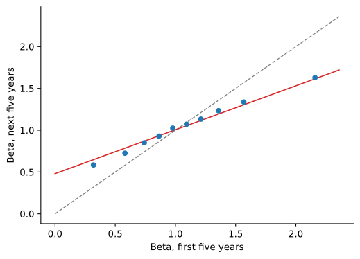
A better forecast of a stock’s future beta therefore shrinks the estimate toward the average, as in Estimation Risk and Shrinkage. Vasicek (1973) derives how far to shrink. If the true betas across stocks are normally distributed with mean \bar{\beta} and variance \sigma_{\beta}^{2}, and the OLS estimate adds normal sampling error to the true beta, the estimate of a stock’s beta with the smallest expected squared error, given its OLS estimate, is \beta_{i}^{V} = w_{i} \hat{\beta}_{i} + (1 - w_{i}) \bar{\beta}, \qquad w_{i} = \frac{\sigma_{\beta}^{2}}{\sigma_{\beta}^{2} + \text{SE}^{2}(\hat{\beta}_{i})}. \tag{11} The weight on the estimate compares the dispersion of betas across stocks with the stock’s own standard error, here the one of (9), so each estimate is shrunk according to its precision. Both parameters come from the cross-section: \bar{\beta} is the average estimated beta, and since each estimate adds sampling error to the true beta, \sigma_{\beta}^{2} is the variance of the estimates minus the average squared standard error. Among the 500 largest stocks over the ten years of Table 3, the estimated betas average 1.04 with a standard deviation of 0.43, and the standard deviation of the true betas is about 0.40. Tesla’s beta gets a weight of 0.60 and shrinks from 2.04 to 1.64, while BlackRock’s, estimated much more precisely, keeps a weight of 0.96.

Vasicek, Oldrich A. 1973. “A Note on Using Cross-Sectional Information in Bayesian Estimation of Security Betas.” Journal of Finance 28 (5): 1233–39.

Blume, Marshall E. 1971. “On the Assessment of Risk.” Journal of Finance 26 (1): 1–10.

Commercial data services use a simpler rule, the adjusted beta \beta_{\text{adj}} = \tfrac{2}{3} \hat{\beta} + \tfrac{1}{3} \times 1, \tag{12} which pulls every estimate one third of the way toward one. The weight goes back to Blume (1971), who regressed the betas of NYSE stocks on their estimates over the previous seven years. His slopes range from about 0.5 to 0.75, and for 1954–1961 on 1947–1954 the regression is 0.343 + 0.677 \hat{\beta}, close to (12). Vasicek’s objection is that a single weight shrinks precise estimates too much and noisy ones too little.

Vasicek’s estimate corrects only for noise, and that is not enough. Over the five-year windows of Figure 3, Vasicek’s weights average 0.78, so his estimate moves betas about 22% of the way toward the mean, while the data move about half of the way. Estimation noise accounts for only about 24% of the cross-sectional variance of the estimated betas. The rest of the pull is real: Blume (1975) finds that firms with extreme betas tend to become less extreme over time, so part of the regression toward one reflects true changes in betas rather than noise. Averaged over all stock-windows, the squared difference between the forecast and the beta estimated over the next five years is 0.254 with the OLS estimate, 0.207 with Vasicek’s and 0.195 with the adjusted beta (12).

Blume, Marshall E. 1975. “Betas and Their Regression Tendencies.” Journal of Finance 30 (3): 785–95.

Levi, Yaron, and Ivo Welch. 2017. “Best Practice for Cost-of-Capital Estimates.” Journal of Financial and Quantitative Analysis 52 (2): 427–63.

Dimson, Elroy. 1979. “Risk Measurement When Shares Are Subject to Infrequent Trading.” Journal of Financial Economics 7 (2): 197–226.

The ten years of monthly returns in Table 3 keep the examples simple, but current practice estimates betas differently. Levi and Welch (2017) study forecasts of next year’s beta for U.S. stocks and recommend three steps. First, estimate betas from one to four years of daily returns. A year of daily returns has about 250 observations, four times as many as five years of monthly returns, so if returns are independent over time, (9) makes the standard error about half as large, and a short window keeps up with a beta that changes over time. Second, shrink the estimate as in (11). Third, since true betas drift toward the mean, shrink the Vasicek estimate a second time, by another 20% to 30%. For betas estimated from three to five years of monthly returns, as in Figure 3, they find that shrinking about halfway toward the mean forecasts best, the same pull as in (10). They also find that the correction of Dimson (1979) for shares that trade infrequently, which adds lagged and leading market returns to the regression and sums their slopes, makes the forecasts worse.

Implications of the Model

The assumption that the residuals of different stocks are uncorrelated cannot hold for two securities whose returns are perfectly correlated, such as a stock and a leveraged position in it. If R_{B} = w R_{A} with w \neq 0, then e_{B} = w e_{A} and \operatorname{Cov}(e_{A}, e_{B}) = w \sigma^{2}(e_{A}), which is not zero as long as A has firm-specific risk. In the following, when we talk about two different assets it is implicitly assumed that their excess returns are not perfectly correlated, unless stated otherwise.

Covariance Structure

The covariance of the excess returns between securities i and j is \operatorname{Cov}(R_{i}, R_{j}) = \operatorname{Cov}(\alpha_{i} + \beta_{i} R_{M} + e_{i}, \alpha_{j} + \beta_{j} R_{M} + e_{j}) = \beta_{i} \beta_{j} \operatorname{Cov}(R_{M}, R_{M}) = \beta_{i} \beta_{j} \sigma_{M}^{2}. \tag{13} The previous expression says that in the single index model, the covariance between any two different securities is given by their exposures to the market and the variance of the market. Dividing by \sigma_{i} \sigma_{j} and using (6), \rho_{i, j} = \frac{\beta_{i} \beta_{j} \sigma_{M}^{2}}{\sigma_{i} \sigma_{j}} = \frac{\sigma_{i} \rho_{i, M}}{\sigma_{M}} \, \frac{\sigma_{j} \rho_{j, M}}{\sigma_{M}} \, \frac{\sigma_{M}^{2}}{\sigma_{i} \sigma_{j}} = \rho_{i, M} \rho_{j, M}. \tag{14} Therefore, in the single-index model, all pairwise correlations between two assets can be computed as the product of their correlations with the market.

Together with the variance decomposition (2), the covariances give the whole covariance matrix of N securities, \pmb{\Sigma} = \sigma_{M}^{2} \pmb{\beta} \pmb{\beta}^{\top} + \mathbf{D}, \tag{15} where \pmb{\beta} is the vector of betas and \mathbf{D} the diagonal matrix of residual variances \sigma^{2}(e_{i}). This is the payoff promised in the introduction. For 500 stocks, the matrix needs 500 betas, 500 residual variances and the market variance, 1{,}001 estimates instead of 125{,}250. The matrix is biased whenever residuals are in fact correlated, since it sets every residual covariance to zero, but it is far more precise than the sample matrix. In Estimation Risk and Shrinkage, minimum-variance portfolios of the 100 largest U.S. stocks built from (15) are far less volatile out of sample than portfolios built from the sample covariance matrix.

The risk of a portfolio does not even need the matrix. A portfolio with weights w_{i} in the N securities, and the rest of its capital in the risk-free asset, has the excess return R_{P} = \alpha_{P} + \beta_{P} R_{M} + \sum_{i} w_{i} e_{i}, and since the residuals are uncorrelated, \sigma_{P}^{2} = \beta_{P}^{2} \sigma_{M}^{2} + \sum_{i=1}^{N} w_{i}^{2} \sigma^{2}(e_{i}), \qquad \beta_{P} = \sum_{i=1}^{N} w_{i} \beta_{i}. \tag{16} The betas and residual variances of the holdings, 2N + 1 numbers with the market variance, say how risky the portfolio is and how much of that risk is the market’s. The same formula gives the risk of a portfolio relative to a benchmark: with the active weights w_{i} - w_{i}^{B} in place of w_{i}, it gives the variance of the difference between the two portfolios’ returns, the squared tracking error. A short position of \beta_{P} in the market removes the first term and leaves only firm-specific risk, which is how a fund hedges the market risk of its holdings (Problem 11).

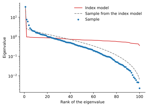
Figure 4 shows where the gain comes from. Standardize each stock’s excess return to a volatility of one. The eigenvalues of the correlation matrix are then the variances of N uncorrelated portfolios of these returns, each scaled so that its squared weights add up to one, and they add up to N. Because the returns are excess returns, the weights need not add up to one: the rest of the capital is in the risk-free asset. The scaling fixes the size of each portfolio, so that it would have a variance of one if returns were uncorrelated (Problem 5 works through an example). Take the 100 largest U.S. stocks at the end of 2015 that have returns in every month of the following ten years, one share class per firm. In the index model fitted to their returns, the largest eigenvalue, essentially the market, is 30.3, and the other 99 lie between 0.35 and 0.97, the smallest and the largest share of firm-specific variance among the stocks. The sample correlation matrix of the same returns has a largest eigenvalue of 33.9, close to the model’s, but the others spread from 7.6 down to 0.002.

How much of that spread is noise? Suppose the fitted index model were the truth, draw 120 months of normal returns from it, and compute the eigenvalues of the sample correlation matrix. On average over 200 draws, the eigenvalues after the first spread from 2.6 down to 0.006, although in the model they all lie in that narrow range. Estimation stretches the spectrum in both directions. The actual eigenvalues have the same shape, stretched further. A few large ones are well above the simulated ones, which points to comovement that the market does not explain, such as within industries (see Beyond a Single Index). Since the eigenvalues add up to N, the others must be lower on average, and in fact most of them lie below the simulated ones. A small eigenvalue belongs to a portfolio that looks nearly riskless in the sample. In the simulation, the smallest sample eigenvalue averages 0.006, while under the model no portfolio of this size has a variance below 0.35.

Figure 4: Eigenvalues, largest first, of the correlation matrix of monthly excess returns of the 100 largest U.S. stocks, January 2016 to December 2025, estimated from the sample and implied by the index model fitted to the same returns, and the average eigenvalues of sample correlation matrices of 120 months of normal returns drawn from the index model. The vertical axis is logarithmic.

Does this noise matter to an investor who cares about expected returns as well as risk? It matters to one who has views about them. An investor who believes every alpha is zero should hold the market and needs no covariance matrix at all. An investor with alphas to exploit needs the whole matrix, to size each bet against the risk it adds, as the Treynor-Black model does. A simulation measures what an estimated matrix costs this investor, because in a simulation we choose the true parameters and can check any portfolio against them.

The truth cannot be the index model itself, or the index model would win by construction. We take the index model fitted to the 100 stocks and add the comovement it misses. The first 5 principal components of its residuals, the source of the few large eigenvalues in Figure 4, become 5 residual factors, uncorrelated with the market and with each other, which explain 38% of the residual variance. The alphas come from these factors, as alphas relative to the CAPM from characteristics such as value or profitability would: each factor earns a Sharpe ratio of 0.3 a year, and a stock’s alpha is its loadings on the factors times their premia. The market premium is 6% a year. The investor knows the expected returns \pmb{\mu}, alphas included, but does not know the true covariance matrix \pmb{\Sigma}. We draw 120 months of normal returns from the true model, independent across months, the investor estimates a covariance matrix \hat{\pmb{\Sigma}} from them, and then holds the portfolio with the highest Sharpe ratio according to that estimate, the tangency portfolio with weights \mathbf{w} proportional to \hat{\pmb{\Sigma}}^{-1} \pmb{\mu}.

A portfolio with weights \mathbf{w} has an expected excess return of \mathbf{w}^{\top} \pmb{\mu}, which the investor knows, and a volatility, which the investor can only estimate. That gives two Sharpe ratios for the same portfolio, \hat{\mathit{SR}} = \frac{\mathbf{w}^{\top} \pmb{\mu}}{\sqrt{\mathbf{w}^{\top} \hat{\pmb{\Sigma}} \mathbf{w}}} \qquad \text{and} \qquad \mathit{SR} = \frac{\mathbf{w}^{\top} \pmb{\mu}}{\sqrt{\mathbf{w}^{\top} \pmb{\Sigma} \mathbf{w}}}, \tag{17} which differ only in the covariance matrix. The first, the investor’s estimate, measures the portfolio’s risk with the estimated matrix. The second, the true value, measures it with the true matrix, which generates the portfolio’s returns. We can compute the true value only because we know \pmb{\Sigma}; a real investor never sees it. With the true matrix, the best portfolio, \pmb{\Sigma}^{-1} \pmb{\mu}, has a Sharpe ratio of 0.74, against 0.38 for the market, so the alphas nearly double what the market offers. We repeat the experiment 500 times, for three covariance matrices the investor might use: the sample covariance matrix; the index model fitted to the same 120 months, that is, (15) with estimated betas, residual variances and market variance; and a five-factor matrix that adds to the index model the first five principal components of the sample’s residuals, in the spirit of Fan et al. (2013). The five-factor investor knows how many residual factors there are, but not what they are. Table 4 reports the averages.

Table 4: Annualized Sharpe ratios (17) of the tangency portfolio of the 100 stocks, averaged over 500 samples of 120 months drawn from the index model with 5 residual factors that carry the alphas. The investor knows the expected returns and estimates the covariance matrix. Both columns give the Sharpe ratio of the same portfolio, before any returns are realized: the investor’s estimate \hat{\mathit{SR}} measures its risk with the investor’s matrix, and the true value \mathit{SR} with the true one. The best attainable Sharpe ratio is 0.74.

Matrix the investor uses	Investor’s estimate	True value
Sample	1.91	0.30
Index model fitted to the sample	1.82	0.63
Five-factor model fitted to the sample	1.03	0.64

With the sample covariance matrix, the investor’s estimate of the Sharpe ratio is 1.91, while its true value is 0.30, less than half of the 0.74 that was available. Noise rotates the eigenvectors of the sample covariance matrix, so the expected returns have small components along the eigenvectors with the smallest eigenvalues, and those eigenvalues are too small, for the same reason as the correlation eigenvalues in Figure 4. The inverse matrix divides each component by its eigenvalue, and small components divided by tiny eigenvalues become large positions. The portfolio fills up with zero-cost positions that look nearly riskless in the sample but carry real firm-specific risk, and that earn little relative to that risk. The estimated volatility of the portfolio is far too low, and so the investor’s estimate of the Sharpe ratio is far too high.

With the index model fitted to the same data, the true value is 0.63, 85% of the best, although the model ignores the residual factors that produce every alpha. The model rules out the positions that look riskless, since under it a zero-cost position that hedges the market still bears the firm-specific risk \sum_{i} w_{i}^{2} \sigma^{2}(e_{i}) of its stocks. Its error is a bias, not noise, and here the bias costs far less. The bias shows in the investor’s estimate, 1.82. The model treats the residual factors as firm-specific risk that diversifies away, so the investor sees the alpha bets as nearly riskless and expects 2.9 times the true Sharpe ratio. The five-factor matrix sees the factors, and its investor’s estimate falls to 1.03, but its true value, 0.64, is barely higher. Imposing the market’s structure does most of the work. The residual factors matter for how much risk the investor believes the portfolio has, much less for the portfolio itself. That belief is not harmless: an investor who targets a level of risk, or a manager with a budget for tracking error, scales the bets by the estimated risk, and an underestimate means positions that are too large. This is the main reason practitioners forecast risk with multifactor models, which add industry and style factors to the market (see Beyond a Single Index). Estimation Error in the Tangency Portfolio runs the same experiment and shows that an investor who estimates the alphas too, from past returns, loses far more than any covariance matrix can recover.

Beyond a Single Index

The index model is a statistical description of returns, and uncorrelated residuals are only an approximation. Stocks in the same industry share shocks that the market does not capture, such as oil prices for energy companies or interest rates for banks, so their residuals are positively correlated, as Problem 9 illustrates. A model with an index for each common source of risk captures more of the comovement, and Beyond the CAPM develops such multifactor models.

Modern estimators of the covariance matrix keep the index model’s discipline without its strict assumption. Ledoit and Wolf (2003) shrink the sample matrix toward (15), taking a weighted average of the two with a weight estimated from the data, so the data decide how much of the comovement the market misses is worth keeping, without having to choose additional factors. Fan et al. (2013) estimate the factors as principal components of the returns and keep only the residual covariances that are large. Ledoit and Wolf (2017) keep the eigenvectors of the sample matrix and shrink each eigenvalue by its own amount, pushing the small ones up and pulling the large ones down, which counters the spread in Figure 4. In each case, the sample covariance matrix is the starting point, never the answer.

Ledoit, Olivier, and Michael Wolf. 2003. “Improved Estimation of the Covariance Matrix of Stock Returns with an Application to Portfolio Selection.” Journal of Empirical Finance 10 (5): 603–21.

Fan, Jianqing, Yuan Liao, and Martina Mincheva. 2013. “Large Covariance Estimation by Thresholding Principal Orthogonal Complements.” Journal of the Royal Statistical Society: Series B (Statistical Methodology) 75 (4): 603–80.

Ledoit, Olivier, and Michael Wolf. 2017. “Nonlinear Shrinkage of the Covariance Matrix for Portfolio Selection: Markowitz Meets Goldilocks.” Review of Financial Studies 30 (12): 4349–88.

The same regression is also the standard test of the CAPM. The CAPM implies that every security’s alpha is zero when the index is the market portfolio, and CAPM Anomalies runs (1) on portfolios sorted by characteristics to test that prediction.

Practice Problems

These problems give you a chance to practice the concepts introduced in this chapter. Try to solve each one on your own before expanding the solution.

Problem 1 (Counting the Inputs) Ingrid Halvorsen, a quantitative analyst at Halcyon Asset Management, covers a universe of 500 stocks and wants to build mean-variance efficient portfolios from it.

1. How many estimates does she need if she works directly with expected returns, variances, and covariances?
2. How many does she need under the single index model?

Solution

1. She needs 500 expected returns, 500 variances, and 500 \times 499 / 2 = 124{,}750 covariances, a total of 125{,}750 estimates.

2. Under the index model, each stock needs an alpha, a beta, and a residual variance, and the market needs an expected excess return and a variance. That is 3 \times 500 + 2 = 1{,}502 estimates. Every covariance follows from (13), so the model cuts the number of inputs by a factor of more than 80.

Problem 2 (Reading a Regression) A regression of Quillon Robotics’ (QLR) excess returns on the market’s excess returns gives a beta of 1.5 and a residual volatility of \sigma(e_{QLR}) = 35\% a year. The market’s volatility is 18\%.

1. Compute QLR’s systematic variance, total variance, and volatility.
2. What R-squared should the regression report?

Solution

1. By (2), the systematic variance is 1.5^{2} \times 0.18^{2} = 0.0729 and the total variance is 0.0729 + 0.35^{2} = 0.1954, so \sigma_{QLR} = \sqrt{0.1954} \approx 44.2\%.

2. By (5), the R-squared is 0.0729/0.1954 \approx 0.37. The market explains a bit more than a third of QLR’s variance, and the rest is firm-specific.

Problem 3 (Covariances and Portfolios Through Betas) Two stocks in Lena Fischer’s portfolio have the following index model estimates. The market’s volatility is 20\%.

Stock	Beta	Volatility
Corbel Aerospace (CBA)	1.2	40%
Dunmore Utilities (DMU)	0.7	25%

1. Compute the covariance and the correlation between the two stocks implied by the index model. Check the correlation using each stock’s correlation with the market.
2. Compute each stock’s residual variance.
3. Lena holds 60\% in CBA and 40\% in DMU. Compute the portfolio’s beta and volatility using the index model.

Solution

1. By (13), \operatorname{Cov}(R_{CBA}, R_{DMU}) = 1.2 \times 0.7 \times 0.20^{2} = 0.0336, so the correlation is 0.0336/(0.40 \times 0.25) = 0.336. By (6), \rho_{CBA, M} = 1.2 \times 0.20/0.40 = 0.60 and \rho_{DMU, M} = 0.7 \times 0.20/0.25 = 0.56, and (14) gives 0.60 \times 0.56 = 0.336 as well.

2. By (2), \sigma^{2}(e_{CBA}) = 0.16 - 1.2^{2} \times 0.04 = 0.1024 and \sigma^{2}(e_{DMU}) = 0.0625 - 0.7^{2} \times 0.04 = 0.0429.

3. The portfolio beta is 0.6 \times 1.2 + 0.4 \times 0.7 = 1.0. Since the residuals are uncorrelated, the portfolio’s residual variance is 0.6^{2} \times 0.1024 + 0.4^{2} \times 0.0429 = 0.0437, and its variance is 1.0^{2} \times 0.04 + 0.0437 = 0.0837, a volatility of about 28.9\%. The two-asset formula with the covariance from part (a) gives the same answer.

Problem 4 (Building a Covariance Matrix) Aisha Rahman needs a covariance matrix for three stocks to feed into a portfolio optimizer. She uses the index model with a market volatility of 20\% and the following estimates:

Stock	Beta	Residual Volatility
Fernhill Grocers (FHG)	0.8	20%
Gallant Media (GLM)	1.0	25%
Hexley Mining (HXM)	1.5	30%

Compute the full covariance matrix of the three stocks’ excess returns.

Solution

By (2), the variances are 0.8^{2} \times 0.04 + 0.04 = 0.0656, 1.0^{2} \times 0.04 + 0.0625 = 0.1025, and 1.5^{2} \times 0.04 + 0.09 = 0.18. By (13), the covariances are 0.8 \times 1.0 \times 0.04 = 0.032, 0.8 \times 1.5 \times 0.04 = 0.048, and 1.0 \times 1.5 \times 0.04 = 0.06. In the order FHG, GLM, HXM, \pmb{\Sigma} = \begin{pmatrix} 0.0656 & 0.032 & 0.048 \\ 0.032 & 0.1025 & 0.06 \\ 0.048 & 0.06 & 0.18 \end{pmatrix}. With three stocks the model needs seven inputs for six distinct entries, so it saves nothing yet. The savings come with size, as Problem 1 shows for 500 stocks.

Problem 5 (Risk in Units of Stocks) A market has N = 100 stocks, and every pair has a correlation of \rho = 0.3. Standardize each stock’s excess return to a volatility of one, so that the correlation matrix \mathbf{C} is also the covariance matrix of the vector \mathbf{x} of standardized returns, and a portfolio \mathbf{w} has return \mathbf{w}^{\top} \mathbf{x}. Since these are excess returns, the weights need not add up to one: the rest of the capital is in the risk-free asset. Consider only portfolios whose squared weights add up to one, so that a portfolio’s variance cannot be raised by scaling it up.

1. The market portfolio \mathbf{m} puts a weight of 1/\sqrt{100} = 0.1 in every stock. Compute its variance.
2. Portfolio \mathbf{h} is long stock 1 and short stock 2, with weights 1/\sqrt{2} and -1/\sqrt{2}. Compute its variance and its covariance with \mathbf{m}.
3. Show that \mathbf{m} is an eigenvector of \mathbf{C} with eigenvalue 1 + (N - 1) \rho, and that every portfolio whose weights add up to zero, like \mathbf{h}, is an eigenvector with eigenvalue 1 - \rho. Check that the eigenvalues add up to N.
4. Suppose returns follow the index model and every stock has the same correlation with the market. What correlation with the market produces \rho = 0.3, and what share of each stock’s variance is firm-specific? Compare with the eigenvalues in (c).

Solution

1. Each of the 100 variances is one and each of the 100 \times 99 covariances is 0.3, so \operatorname{V}(\mathbf{m}^{\top} \mathbf{x}) = 0.1^{2} \times (100 + 100 \times 99 \times 0.3) = 1 + 99 \times 0.3 = 30.7. This one portfolio carries the risk of 30.7 stocks.
2. \operatorname{V}(\mathbf{h}^{\top} \mathbf{x}) = \tfrac{1}{2} (1 + 1 - 2 \times 0.3) = 1 - 0.3 = 0.7. Every stock has the same covariance with \mathbf{m}, namely 0.1 \times (1 + 99 \times 0.3), so a long position in one stock and an equal short position in another cancel, and \operatorname{Cov}(\mathbf{h}^{\top} \mathbf{x}, \mathbf{m}^{\top} \mathbf{x}) = 0. The long-short portfolio hedges out the market.
3. Write \mathbf{C} = (1 - \rho) \mathbf{I} + \rho \mathbf{1} \mathbf{1}^{\top}. Then \mathbf{C} \mathbf{m} = (1 - \rho) \mathbf{m} + \rho \mathbf{1} (\mathbf{1}^{\top} \mathbf{m}) = (1 - \rho) \mathbf{m} + \rho N \mathbf{m} = (1 + (N - 1) \rho) \mathbf{m}, since \mathbf{1}^{\top} \mathbf{m} = N / \sqrt{N} and \mathbf{1} = \sqrt{N} \mathbf{m}. For weights \mathbf{w} with \mathbf{1}^{\top} \mathbf{w} = 0, \mathbf{C} \mathbf{w} = (1 - \rho) \mathbf{w}. The weights that add up to zero form a space of dimension N - 1 = 99, so the eigenvalues are 30.7 once and 0.7 ninety-nine times, and 30.7 + 99 \times 0.7 = 100 = N, the sum of the diagonal of \mathbf{C}. Correlation does not create or destroy risk. It decides how the 100 units are shared between the market and the hedged portfolios.
4. By (14), \rho = \rho_{i, M}^{2}, so \rho_{i, M} = \sqrt{0.3} = 0.548. The R-squared of each stock is 0.3, and the firm-specific share of its variance is 1 - 0.3 = 0.7, exactly the eigenvalue of the hedged portfolios. Hedging out the market leaves only firm-specific risk. With different correlations with the market, the 99 small eigenvalues spread between the smallest and largest firm-specific shares, as in Figure 4.

Problem 6 (How Many Stocks Are Enough?) Marcus Bell builds equally weighted portfolios from a universe of stocks, each with a beta of 1.1 and a residual volatility of 40\%. The market’s volatility is 20\%, and the index model holds.

1. Compute the volatility of an equally weighted portfolio of 10 stocks and of 50 stocks.
2. What volatility does the portfolio approach as the number of stocks grows without bound?
3. How many stocks does Marcus need for the portfolio’s volatility to be within one percentage point of that limit?

Solution

1. An equally weighted portfolio of N stocks has beta 1.1 and, with uncorrelated residuals, residual variance 0.16/N. Its variance is 1.1^{2} \times 0.04 + 0.16/N = 0.0484 + 0.16/N. With N = 10 that is 0.0644, a volatility of about 25.4\%; with N = 50 it is 0.0516, about 22.7\%.

2. As N grows, the residual variance vanishes and the volatility approaches \sqrt{0.0484} = 22\%, the systematic risk \beta \sigma_{M} = 1.1 \times 20\%.

3. Marcus needs 0.0484 + 0.16/N \le 0.23^{2} = 0.0529, or N \ge 0.16/0.0045 \approx 35.6, so 36 stocks.

Problem 7 (Estimating a Beta by Hand) Sam Okoro, an intern at Brightline Advisors, has five months of excess returns, in percent, for Tamarind Foods (TMF) and the market:

Month	Market	TMF
1	3	3
2	-1	-3
3	5	9
4	-3	-3
5	1	4

Use (3) and (4) to estimate TMF’s beta and alpha, and compute the R-squared of the regression.

Solution

The averages are 1\% for the market and 2\% for TMF. The deviations from the averages are (2, -2, 4, -4, 0) for the market and (1, -5, 7, -5, 2) for TMF. The sum of products of deviations is 2 + 10 + 28 + 20 + 0 = 60, and the sum of squared market deviations is 4 + 4 + 16 + 16 + 0 = 40. The common divisor cancels in the ratio, so \beta_{TMF} = \frac{60}{40} = 1.5, \qquad \alpha_{TMF} = 2 - 1.5 \times 1 = 0.5\%. The sum of squared TMF deviations is 1 + 25 + 49 + 25 + 4 = 104, so by (7) \text{R-squared} = \rho^{2} = \frac{60^{2}}{40 \times 104} \approx 0.87. Five observations are far too few for reliable estimates, which is why the example in this note uses ten years of monthly data.

Problem 8 (Is the Alpha Real?) A regression of Elmstead Pharmaceuticals’ (EPH) monthly excess returns on the market’s gives an alpha of 0.5\% per month with a p-value of 0.30, and a beta of 1.3. The market’s expected excess return is 0.6\% per month.

1. Using the point estimates, what is EPH’s expected excess return per month?
2. A colleague, Ruth Abernathy, says EPH beats the market by half a percent a month. How would you respond?
3. Suppose the alpha is real. Fairmont Devices (FMD) has the same alpha of 0.5\% per month, but a residual volatility of 4\% per month against EPH’s 12\%. Which alpha is more valuable? How should the positions in the two stocks compare?

Solution

1. Taking expectations in (1), \operatorname{E}(R_{EPH}) = 0.5\% + 1.3 \times 0.6\% = 1.28\% per month.

2. Most of EPH’s expected excess return comes from its market exposure, which any investor can get by holding the market with leverage. The alpha is the only part that would beat the market, and with a p-value of 0.30 we cannot reject that it is zero. A positive point estimate of this size is common even when the true alpha is zero, so the regression gives no reliable evidence that EPH beats the market.

3. By (8), EPH’s information ratio is 0.5/12 \approx 0.04 and FMD’s is 0.5/4 = 0.125, so FMD’s alpha is the better one: it comes with a third of the firm-specific risk. Positions proportional to \alpha_{i}/\sigma^{2}(e_{i}) give FMD (12/4)^{2} = 9 times the weight of EPH.

Problem 9 (When the Residuals Are Correlated) Two regional banks, Harrow Bank (HRW) and Penfold Bank (PNF), have correlations with the market of 0.7 and 0.5. Over the same period, the sample correlation between their excess returns is 0.6.

1. What correlation does the single index model predict?
2. What does the gap say about the residuals of the two banks, and why might it arise?
3. Would the index model overstate or understate the risk of a portfolio made only of bank stocks?

Solution

1. By (14), the model predicts 0.7 \times 0.5 = 0.35.

2. The observed correlation is higher, so the residuals of the two banks are positively correlated, contradicting the assumption that \operatorname{Cov}(e_{i}, e_{j}) = 0. Banks share exposures beyond the market, such as interest rates, credit conditions, and regulation, and these industry shocks show up in both residuals.

3. The model would understate it. It treats the residuals as diversifiable across the banks, but shocks common to the industry do not average out within a portfolio of banks.

Problem 10 (Two Undervalued Stocks) Carla Mendoza is comparing two stocks that her analysis says are undervalued. Tidewell Shipping (TWS) has an alpha of 3\% and a residual volatility of 15\%. Brightfold Bio (BFB), a small biotech, has an alpha of 8\% and a residual volatility of 60\%.

1. Compute each stock’s information ratio and compare the positions \alpha_{i}/\sigma^{2}(e_{i}) that the two stocks deserve.
2. Carla doubles her investment in BFB. What happens to the alpha, the residual volatility and the information ratio of her BFB position?
3. Suppose there were N biotechs like BFB, each with an alpha of 8\% and a residual volatility of 60\%, with independent residuals. How many, held in equal weights, would match the information ratio of TWS?

Solution

1. By (8), the information ratios are 0.03/0.15 = 0.2 for TWS and 0.08/0.60 = 0.13 for BFB. The positions are 0.03/0.15^{2} = 1.33 and 0.08/0.60^{2} = 0.22, so TWS deserves 6 times the weight, although its alpha is less than half of BFB’s. The larger mispricing is the worse opportunity.

2. Measured in dollars, the alpha and the residual risk of the position both double, so the information ratio stays at 0.13. A bigger position in one stock scales the reward and the risk together.

3. An equally weighted portfolio of N such stocks has an alpha of 8\% and a residual volatility of 60\%/\sqrt{N}, so its information ratio is 0.133 \sqrt{N}. It reaches 0.2 when \sqrt{N} = 1.5, or N = 2.25, so three stocks are enough, with an information ratio of 0.133 \sqrt{3} = 0.23. Diversification needs different firms with independent firm-specific risk, not more shares of the same one.

Problem 11 (Hedging Out Market Risk) Garnet Capital, a hedge fund, buys $10 million of Lumen Optics (LMO). Its analysts estimate an alpha of 2\% a year, a beta of 1.4, and a residual volatility of 25\% a year. The fund’s manager, Tomas Varga, wants a bet on LMO’s alpha alone, without exposure to the market.

1. How large a short position in an S&P 500 index fund should Tomas take?
2. What are the expected excess dollar return and the dollar volatility of the hedged position over a year?

Solution

1. The position’s beta is zero when the dollar beta of the short matches that of the long: 1.4 \times \$10 \text{ million} = \$14 million short in the index fund.

2. With the market exposure removed, (1) leaves the excess return \$10 \text{ million} \times (\alpha_{LMO} + e_{LMO}). The expected excess return is 0.02 \times \$10 \text{ million} = \$200{,}000, and the dollar volatility is 0.25 \times \$10 \text{ million} = \$2.5 million. The hedge removes market risk but leaves a large firm-specific risk relative to the expected gain, which is why funds spread their alpha bets across many stocks.

Problem 12 (How Precise Is a Beta?) Priya Nair estimates the beta of Kestrel Semiconductors (KSC) from 60 months of returns and gets 1.6. The residual volatility is 10\% a month, and the market’s volatility is 4.5\% a month.

1. Use (9) to compute the standard error of the estimate and a 95% confidence interval for KSC’s beta.
2. Compute the adjusted beta with (12), and the forecast of next period’s beta implied by a regression like (10) with an intercept of 0.5 and a slope of 0.5.
3. With a market risk premium of 6\%, what expected excess return does the CAPM give with each of the three betas?

Solution

1. \text{SE}(\hat{\beta}) = 0.10 / (0.045 \times \sqrt{60}) = 0.29, so the interval is 1.6 \pm 1.96 \times 0.29, from 1.04 to 2.16. Five years of data leave the beta very uncertain, because KSC’s firm-specific risk is large relative to the market’s.

2. \beta_{\text{adj}} = \tfrac{2}{3} \times 1.6 + \tfrac{1}{3} = 1.40, and the regression gives 0.5 + 0.5 \times 1.6 = 1.30.

3. 1.6 \times 6\% = 9.6\%, 1.4 \times 6\% = 8.4\% and 1.3 \times 6\% = 7.8\%. The choice of beta moves the cost of equity by almost two percentage points, more than many of the adjustments analysts argue about.