Forward Rates
Today’s zero-coupon bond prices fix more than today’s interest rates. By combining bonds of different maturities, an investor can lock in today the rate at which money will be lent or borrowed between two future dates. That rate is the forward rate. This chapter shows how to synthesize forward rates from zero-coupon bonds, what the forward curve looks like in the Treasury market, and how forward rates relate to the short rates that investors expect. The gap between the two, the term premium, organizes the traditional theories of the term structure.
Synthesizing Forward Rates
The term structure of interest rates allows investors to lock future interest rates using forward-rates that can be synthesized from zero-coupon rates.
Denote by Z(n) the price of a zero-coupon bond with face value equal to $1 and expiring at year n. Consider now two zero-coupon bonds with expirations m < n, that we will denote by M and N, respectively.
Let’s see what happens if we sell \frac{Z(n)}{Z(m)} units of bond M and invest the proceeds in bond N. The proceeds from selling \frac{Z(n)}{Z(m)} units of M are the number of units times the price per unit, i.e., \frac{Z(n)}{Z(m)} \times Z(m) = Z(n). Therefore, by selling \frac{Z(n)}{Z(m)} units of M you get the amount needed to buy 1 unit of bond N.
The table below describes the cash flows from this strategy, where a negative sign is used to indicate that you pay a certain amount, and a positive sign indicates that you are receiving that amount.
| Year | 0 | m | n |
|---|---|---|---|
| Sell \frac{Z(n)}{Z(m)} units of M | Z(n) | -\frac{Z(n)}{Z(m)} | 0 |
| Buy 1 unit of N | -Z(n) | 0 | 1 |
| Total | 0 | -\frac{Z(n)}{Z(m)} | 1 |
The table shows that this strategy creates a forward-starting zero-coupon bond. Instead of investing a certain amount today at a known interest rate, and therefore guaranteeing a known amount at maturity, this newly created security guarantees today that if you invest a certain amount in year m, you will earn a known interest rate from year m to year n.
The implicit annualized interest rate f(m, n) that applies to this newly created security is called the forward-rate from year m to n, which must satisfy \frac{1}{(1 + f(m, n))^{(n - m)}} = \frac{Z(n)}{Z(m)}, so that f(m, n) = \left( \frac{Z(m)}{Z(n)} \right)^{\!\frac{1}{n - m}} - 1. \tag{1}
Example 1 (Computing Forward Rates) Suppose that we have the following information on zero-coupon bonds for various maturities:
| Bond | Maturity (years) | Price ($) |
|---|---|---|
| Z_{1} | 1 | 920 |
| Z_{2} | 2 | 840 |
| Z_{3} | 3 | 760 |
| Z_{4} | 4 | 710 |
- The forward rate f(2, 4) that applies from years 2 to 4 satisfies f(2, 4) = \left(\frac{840}{710}\right)^{\!1/2} - 1 = 8.77\%.
- The forward rate f(1, 4) that applies from years 1 to 4 satisfies f(1, 4) = \left(\frac{920}{710}\right)^{\!1/3} - 1 = 9.02\%.
- The forward rate f(3, 4) that applies from years 3 to 4 satisfies f(3, 4) = \frac{760}{710} - 1 = 7.04\%.
Sometimes, the forward rate is expressed as a function of the zero-coupon rates implicit in the zero-coupon bond prices. If we denote by r(m) and r(n) the zero-coupon rates corresponding to maturities m and n, respectively, Equation (1) can be re-written as f(m, n) = \left( \frac{(1 + r(n))^{n}}{(1 + r(m))^{m}} \right)^{\!\frac{1}{n - m}} - 1. \tag{2}
Note that if we could fix the forward rate f(m, n) beforehand, then it must be the case that investing from 0 to m at r(m), and then rolling the deposit from m to n at f(m, n), should be equivalent to investing all the way from 0 to n at r(n). If not, there would be a simple arbitrage opportunity where we could invest using the strategy that delivers the most and borrow using the other alternative.
Therefore, it must be the case that: (1 + r(m))^{m} (1 + f(m, n))^{n - m} = (1 + r(n))^{n}, which also delivers equation (2).
Example 2 (One-Year Forward Rates) The table below shows the zero-coupon rate per year compounded annually for different maturities. The forward rate that applies from the previous to the current year is computed in the last column.
| Year | Zero Rate (%) | Forward Rate (%) |
|---|---|---|
| 1 | 4.0 | |
| 2 | 5.0 | 6.01 |
| 3 | 5.6 | 6.81 |
| 4 | 6.0 | 7.21 |
| 5 | 6.3 | 7.51 |
In the table, the forward rate that applies from year 1 to 2 is computed as f(1, 2) = \frac{1.05^{2}}{1.04} - 1 = 6.01\%, whereas the forward rate that applies from year 4 to 5 is given by f(4, 5) = \frac{1.063^{5}}{1.06^{4}} - 1 = 7.51\%.
Forward Rates with Continuous Compounding
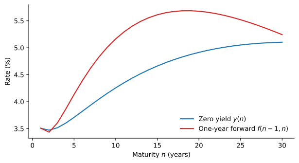
With continuously compounded zero yields y_{t}(n), as in Bond Pricing, the condition that rolling a deposit from m to n at the forward rate matches investing until n becomes e^{m y_{t}(m)} e^{(n - m) f_{t}(m, n)} = e^{n y_{t}(n)}, so the continuously compounded forward rate is f_{t}(m, n) = \frac{n \, y_{t}(n) - m \, y_{t}(m)}{n - m}. \tag{3} The formula has a simple reading. Since n \, y_{t}(n) = m \, y_{t}(m) + (n - m) f_{t}(m, n), the yield to maturity n is the average of the forward rates over the life of the bond. In particular, with one-year forward rates, y_{t}(n) = \frac{1}{n} \sum_{k=0}^{n-1} f_{t}(k, k+1), \qquad f_{t}(0, 1) = y_{t}(1). \tag{4} When the yield curve slopes upward, each new forward rate is above the average of the previous ones, so the forward curve lies above the yield curve. When the yield curve slopes downward, the forward curve lies below it.
Figure 1 shows the zero yields and the one-year forward rates implied by the Treasury yield curve at the end of 2025. Apart from a small dip between one and two years, the curve was upward sloping, so the forward rates lie above the zero yields. The one-year rate was 3.51%, but the forward rate for the year from 9 to 10 was 5.16%. The forward rates peak at about 5.7% near 19 years and then decline slowly as the yield curve flattens.
Forward Rates, Expected Rates and Term Premia
A forward rate is a rate that can be locked in today. Whether it is also a forecast of the rate that will prevail in the future depends on what investors require for holding long-term bonds. Write the one-year forward rate for the year from n - 1 to n as the expected one-year rate in n - 1 years plus a term premium, where all rates are continuously compounded. The equation defines the term premium as whatever separates the forward rate from the expected future rate, apart from a small convexity effect discussed below.
The term premium is also the expected excess return of a long-term bond. Buy a 2-year zero-coupon bond at time t and sell it a year later, when it has become a 1-year bond. Since \ln Z_{t}(n) = -n \, y_{t}(n), as in Bond Pricing, the log return is \ln Z_{t+1}(1) - \ln Z_{t}(2) = 2 y_{t}(2) - y_{t+1}(1), and in excess of the one-year yield y_{t}(1) it is \mathit{rx}_{t+1}(2) = 2 y_{t}(2) - y_{t}(1) - y_{t+1}(1) = f_{t}(1, 2) - y_{t+1}(1), \tag{6} using (3). The bond beats the one-year deposit exactly when next year’s one-year rate turns out below today’s forward rate. Taking expectations, the expected excess log return of the 2-year bond is f_{t}(1, 2) - \operatorname{E}_{t}(y_{t+1}(1)) = \mathit{TP}_{t}(2). A positive term premium is compensation for holding a bond whose price falls when rates rise.
The traditional theories of the term structure are statements about the term premium.
The Expectations Hypothesis
The expectations hypothesis (EH) holds that the term premium is zero, so forward rates are the market’s forecasts of future short rates, and every bond has the same expected return over the next year. In a world populated by risk-neutral investors, the expected holding-period return of investing in any asset should be the risk-free zero rate that applies to that period.
Denote by B the price of a bond paying annual coupons C and expiring at time T. If the expectations hypothesis holds, the expected HPR of buying this bond at time 0 for B_{0} and selling it next year for B_{1} must be r_{0}(1), the zero rate at time 0 that applies to cash flows in year 1, \operatorname{E}(R_{1}) = \frac{\operatorname{E}(B_{1}) + C}{B_{0}} - 1 = r_{0}(1). Note that B_{1} is unknown today since we do not know how interest rates will evolve over time.
Example 3 (Computing an Expected Bond Price) Suppose you have the following information on zero-coupon rates.
| Maturity (years) | Rate (%) |
|---|---|
| 1 | 5.0% |
| 2 | 5.5% |
| 3 | 6.0% |
| 4 | 6.3% |
| 5 | 6.5% |
Consider a 4% annual-paying coupon bond over a notional of $1,000 expiring in 5 years. The price of this bond today can be computed by discounting its cash flows at the appropriate zero-rate. B_{0} = \frac{40}{1.05} + \frac{40}{1.055^{2}} + \frac{40}{1.06^{3}} + \frac{40}{1.063^{4}} + \frac{1040}{1.065^{5}} = 898.02
If the EH holds, the price of this bond next year, B_{1}, should be such that \frac{B_{1} + C}{B_{0}} = 1 + r_{0}(1), implying B_{1} = 898.02 \times 1.05 - 40 = \$902.92.
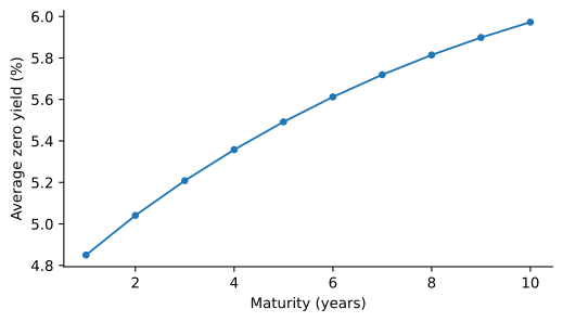
If the EH holds, the shape of the yield curve reflects expected changes in short rates. An upward-sloping curve means the market expects short rates to rise, and a downward-sloping curve that it expects them to fall. Over a long period, short rates rise about as often as they fall, so under the EH the yield curve should be flat on average.
Figure 2 shows that it is not. From 1972 to 2025, the 1-year zero yield started at 4.2% and ended at 3.5%, with no net rise, yet the average yield rises steadily with maturity, from 4.85% at one year to 5.97% at ten years, and the 10-year yield was above the 1-year yield in 81% of the months. Short rates did not rise on average, so the average upward slope points to a positive term premium.
The Liquidity Preference Theory
The EH treats bonds of all maturities as perfect substitutes. When investors are risk averse, they care not only about the expected short rate but also about its volatility. Investors in long-term bonds want to be compensated for committing their funds for a long time, since they face price risk if they need to sell before maturity. Conversely, issuers of bonds are willing to pay a higher interest rate on long-term bonds because they can lock in an interest rate for many years. The liquidity preference theory therefore holds that the term premium is positive and grows with maturity, which explains why the yield curve slopes upward on average. With two years, it implies that r_{0}(2) > \frac{r_{0}(1) + \operatorname{E}(r_{1}(1))}{2}.
Segmented Markets and Preferred Habitat
The segmented markets theory holds that investors at different maturities do not substitute between them at all. Some investors, such as money market funds, hold only short-term bonds, while others, such as pension funds and insurance companies that must match long-term liabilities, hold only long-term bonds, so each segment’s rate is set by supply and demand within it. The softer preferred habitat view lets investors leave their preferred maturities for a high enough premium. In either case the term premium at each maturity depends on the supply of bonds of that maturity relative to the demand for them, and it can change over time as the Treasury changes the maturity of its debt or as the Federal Reserve buys long-term bonds.
The three theories differ only in what they say about \mathit{TP}_{t}(n): zero under the EH, positive and rising with maturity under liquidity preference, and driven by the supply and demand of each maturity under segmented markets. Which is closest to the data is an empirical question, and the answer turns on whether forward rates forecast future short rates or the returns of long-term bonds. The Term Structure in the Data takes it up.
The Convexity Adjustment
Even under the EH, forward rates are not exactly the expected future rates, because bond prices are convex in yields. Our version of the EH is consistent with assuming that expected future discount factors can be computed using forward rates, i.e., \operatorname{E}(Z_{t}(n)) = \operatorname{E}\left(\frac{1}{(1 + r_{t}(n))^{n}}\right) = \frac{1}{(1 + f(t, t+n))^{n}}. \tag{7} We can use equation (7) to derive an expression that relates expected future zero rates and forward rates, here with annual compounding.
The first thing to notice is that Jensen’s inequality implies that \operatorname{E}\left(\frac{1}{(1 + r_{t}(n))^{n}}\right) > \frac{1}{(1 + \operatorname{E}(r_{t}(n)))^{n}}, which combined with (7) delivers \operatorname{E}(r_{t}(n)) > f(t, t + n). Therefore, our version of the EH implies that forward rates are a downward biased estimate of future zero-rates. The difference between the two, however, is in general very small. To see why, consider the function h(x) = \frac{1}{(1 + x)^n}. The second order Taylor expansion of h(x) around x = \mu is: \frac{1}{(1 + x)^n} \approx \frac{1}{(1 + \mu)^n} - n \frac{(x - \mu)}{(1 + \mu)^{n + 1}} + \frac{1}{2} n (n + 1) \frac{(x - \mu)^{2}}{(1 + \mu)^{n + 2}}. \tag{8} Consider now a random variable X such that \operatorname{E}(X) = \mu and \operatorname{V}(X) = \sigma^{2}. Taking expectations on both sides of (8) shows that \operatorname{E}\left(\frac{1}{(1 + X)^n}\right) \approx \frac{1}{(1 + \mu)^n} + \frac{1}{2} n (n + 1) \frac{\sigma^{2}}{(1 + \mu)^{n + 2}}. \tag{9} Denoting f = f(t, t + n), \mu = \operatorname{E}(r_{t}(n)) and \sigma^{2} = \operatorname{V}(r_{t}(n)), we can combine (7) and (9) to obtain \frac{1 + \mu}{1 + f} \approx \left(1 + \frac{1}{2} n (n + 1) \left(\frac{\sigma}{1 + \mu}\right)^{\!2} \right)^{\!1/n}. The previous expression shows that the difference between expected future rates and forward rates depends on a convexity adjustment term on the right of the above expression. For typical values of \mu and \sigma, the convexity adjustment term is very small, which allows us to conclude that if the EH holds, forward rates are good forecasts of expected future zero-rates, i.e., \operatorname{E}(r_{t}(n)) \approx f(t, t+n).
Practice Problems
These problems give you a chance to practice the concepts introduced in this chapter. Try to solve each one on your own before expanding the solution.
Problem 1 (Forward Rates from Zero Prices) Helena Brooks, who runs the Treasury desk at Marlow Securities, sees the following prices for zero-coupon bonds with a face value of $1.
| Maturity (years) | 1 | 2 | 3 | 4 |
|---|---|---|---|---|
| Price ($) | 0.962 | 0.918 | 0.871 | 0.822 |
Compute the forward rates f(1, 2), f(1, 3), f(2, 4), and f(3, 4).
Solution
By (1), \begin{aligned} f(1, 2) & = \frac{0.962}{0.918} - 1 \approx 4.79\%, & f(1, 3) & = \left( \frac{0.962}{0.871} \right)^{\!1/2} - 1 \approx 5.09\%, \\ f(2, 4) & = \left( \frac{0.918}{0.822} \right)^{\!1/2} - 1 \approx 5.68\%, & f(3, 4) & = \frac{0.871}{0.822} - 1 \approx 5.96\%. \end{aligned}Problem 2 (One-Year Forwards and Expected Rates) The zero rates below are expressed per year with annual compounding.
| Maturity (years) | 1 | 2 | 3 | 4 |
|---|---|---|---|---|
| Zero Rate (%) | 3.5 | 4.0 | 4.4 | 4.7 |
- Compute the one-year forward rates f(1, 2), f(2, 3), and f(3, 4).
- If the expectations hypothesis holds, what do these forward rates say about the one-year rate over the next three years?
Solution
By (2), f(1, 2) = \frac{1.04^{2}}{1.035} - 1 \approx 4.50\%, \quad f(2, 3) = \frac{1.044^{3}}{1.04^{2}} - 1 \approx 5.20\%, \quad f(3, 4) = \frac{1.047^{4}}{1.044^{3}} - 1 \approx 5.61\%.
Under the EH, forward rates are approximately the expected future one-year rates, so the market expects the one-year rate to rise from 3.5% today to about 4.50%, 5.20%, and 5.61% in years 1, 2, and 3. The upward-sloping term structure reflects expected increases in short rates.
Problem 3 (Locking In a Future Borrowing Rate) Tolland Freight will need to borrow $5 million in two years for one year to pay for new trucks. Its treasurer, Diego Alvarez, wants to lock in the rate today using zero-coupon bonds priced off the zero rates in Problem 2.
- Which positions in 2-year and 3-year zeros give the firm $5 million in year 2 and a fixed payment in year 3, at zero cost today?
- What borrowing rate does this lock in?
Solution
Buy 2-year zeros with a face value of $5 million, which cost 5{,}000{,}000/1.04^{2} today, and pay for them by selling 3-year zeros with the same present value. Since 1/(1 + f(2, 3)) = Z(3)/Z(2), the 3-year zeros sold have a face value of 5{,}000{,}000 \times (1 + f(2, 3)) \approx \$5{,}260{,}231. In year 2 the firm receives $5 million, and in year 3 it pays $5,260,231.
The firm borrows $5 million in year 2 and repays $5,260,231 in year 3, a rate of f(2, 3) \approx 5.20\%, fixed today.
Problem 4 (A Mispriced Forward Deposit) With the zero rates of Problem 2, Calder Bank offers a forward deposit: a client can commit today to deposit money in one year for one year at a rate of 5%. Show that Rachel Kim, a trader, can earn a riskless profit, and compute it per $1 million deposited.
Solution
The implied forward rate is f(1, 2) \approx 4.50\%, below the bank’s 5%, so the bank’s deposit is too generous. Rachel commits to deposit $1 million with the bank in year 1 and borrows synthetically from year 1 to year 2: she buys 1-year zeros with a face value of $1 million and finances them by selling 2-year zeros with a face value of 1{,}000{,}000 \times 1.0450 \approx \$1{,}045{,}024. The position costs nothing today. In year 1 the 1-year zeros pay $1 million, which she deposits with the bank. In year 2 she receives $1,050,000 from the bank and pays $1,045,024 on the 2-year zeros, a riskless profit of about $4,976.Problem 5 (Two Ways to Invest for Three Years) Sam Okoro wants to invest for three years. He can buy a 3-year zero at the rate in Problem 2, or invest for one year and lock in today the rate for the following two years.
- What forward rate f(1, 3) makes the two strategies equivalent?
- What would happen if a bank offered a two-year forward deposit starting in one year at a higher rate?
Solution
The strategies are equivalent when (1.035)(1 + f(1, 3))^{2} = 1.044^{3}, or f(1, 3) = \left( \frac{1.044^{3}}{1.035} \right)^{\!1/2} - 1 \approx 4.85\%.
Investors would invest for one year and lock in the bank’s rate, funding the position by borrowing at the 3-year rate. That earns a riskless profit, and in competitive markets the bank’s rate would be pushed back to 4.85%.
Problem 6 (The Expected Price of a Coupon Bond) The zero rates are 4% for one year, 4.5% for two years, and 5% for three years, per year with annual compounding. Paloma Ruiz considers a 3-year Penhallow Utilities bond with annual coupons at 6% on a face value of $1,000.
- Compute the bond’s price today.
- If the expectations hypothesis holds, what is the bond’s expected price one year from now, just after its first coupon?
Solution
Discounting each cash flow at its zero rate, B_{0} = \frac{60}{1.04} + \frac{60}{1.045^{2}} + \frac{1{,}060}{1.05^{3}} \approx \$1{,}028.30.
Under the EH, the expected one-year HPR equals the one-year rate, (\operatorname{E}(B_{1}) + 60)/B_{0} = 1.04, so \operatorname{E}(B_{1}) = 1{,}028.30 \times 1.04 - 60 \approx \$1{,}009.44.
Problem 7 (Riding the Yield Curve) With the zero rates of Problem 2, Victor Salgado buys a 2-year zero with a face value of $1 and plans to sell it after one year.
- If the term structure does not change over the year, what is his one-year return? Compare it with the 1-year rate.
- What one-year return does the expectations hypothesis predict, and what must it assume about next year’s one-year rate?
Solution
He pays 1/1.04^{2} \approx 0.92456. If the term structure is unchanged, the bond becomes a 1-year zero priced at 1/1.035 \approx 0.96618, so his return is 0.96618/0.92456 - 1 \approx 4.50\%, well above the 3.5% one-year rate. This strategy is known as riding the yield curve.
Under the EH, every bond is expected to earn the one-year rate of 3.5%. That requires next year’s one-year rate to rise to about f(1, 2) \approx 4.50\%, which lowers the bond’s price next year. Riding the yield curve beats the one-year rate only if rates rise by less than the forward rates predict.
Problem 8 (How Big Is the Convexity Adjustment?) Under the expectations hypothesis, forward rates understate expected future zero rates by a convexity adjustment.
- For a 5-year zero rate with an expected value of 5% and a standard deviation of 1%, compute the forward rate f implied by the approximation in this note, and the gap \mu - f in basis points.
- Repeat for a 10-year rate with an expected value of 5% and a standard deviation of 2%.
Solution
With n = 5, \mu = 0.05, and \sigma = 0.01, \frac{1 + \mu}{1 + f} \approx \left( 1 + \frac{1}{2} \times 5 \times 6 \times \left( \frac{0.01}{1.05} \right)^{\!2} \right)^{\!1/5} \approx 1.00027, so f \approx 4.971\% and the gap is about 3 basis points.
With n = 10 and \sigma = 0.02, the ratio is about 1.00198, so f \approx 4.793\% and the gap is about 21 basis points. The adjustment grows with maturity and volatility, and it is small for short maturities.
Solution
f(1, 2) = 1.05^{2}/1.04 - 1 \approx 6.01\%.
No. Under the EH, the forward rate would be close to the expected rate, but here it exceeds Laura’s forecast by about one percentage point. The liquidity preference theory attributes the gap to a term premium: investors require extra compensation to hold the riskier 2-year bond, so r_{0}(2) = 5\% > (4\% + 5\%)/2 = 4.5\%.
Solution
f(1, 2) = 2 \times 3.6\% - 3.0\% = 4.2\% and f(2, 3) = 3 \times 4.0\% - 2 \times 3.6\% = 4.8\%. The average of 3.0\%, 4.2\% and 4.8\% is 4.0\%, the 3-year yield.
By (5), \mathit{TP}(2) = 4.2\% - 3.6\% = 0.6\%.
The excess log return is f(1, 2) - y_{t+1}(1), so 4.2\% - 3.6\% = 0.6\% if her forecast is right, and 4.2\% - 5\% = -0.8\% if the one-year yield rises to 5%. The term premium is the excess return she expects, not the one she is guaranteed.