Credit Risk and Corporate Bonds
Corporations borrow by issuing bonds that promise fixed payments, like Treasuries, but unlike the Treasury a corporation can fail to pay. A corporate bond is therefore a claim on the cash flows of a firm that is senior to its stock, and its price reflects both the time value of money of Bond Pricing and the risk of default. This chapter asks how much investors are paid for bearing that risk. It separates the promised yield of a corporate bond from its expected return, shows how corporate yield spreads have moved over a century, examines how much of the spread compensates for expected default losses, and measures the returns of corporate bonds since 2002 from transaction prices.
Promised Yields and Expected Returns
The yield of a corporate bond is a promised yield: the return earned if every payment is made on time. Rating agencies such as Moody’s and Standard & Poor’s grade bonds by their risk of default. Bonds rated Baa or BBB and above are investment grade; bonds rated below are high yield, or junk. The difference between a corporate bond’s yield and the yield of a Treasury with the same maturity is its yield spread.
Consider a one-year zero-coupon bond with a promised yield y. With probability \pi the issuer defaults, and bondholders recover a fraction R of the face value. The expected payoff per dollar of face value is (1 - \pi) + \pi R = 1 - \pi (1 - R), so the expected return is \operatorname{E}(r) = (1 + y) \left( 1 - \pi (1 - R) \right) - 1 \approx y - \pi (1 - R). \tag{1} The term \pi (1 - R) is the expected default loss. The spread over Treasuries pays for this expected loss and for anything else that makes investors require a higher expected return on the corporate bond: a risk premium, because defaults cluster in bad times, a liquidity premium, because corporate bonds are costly to trade, and taxes, since the interest on corporate bonds is taxed by states while the interest on Treasuries is not.
Example 1 (How Much of the Spread Is Expected Loss?) One-year Treasuries yield 4.5%. A Baa-rated one-year bond yields 6%, a spread of 1.5 percentage points, and has a default probability of 0.25% with a recovery of 40% of face value. By (1), its expected return is 1.06 \times (1 - 0.0025 \times 0.6) - 1 = 5.84\%, so the expected loss accounts for only 0.16 percentage points of the spread, about a tenth. The other 1.34 points are expected return in excess of Treasuries.
A B-rated one-year bond yields 8.5%, a spread of 4 points, with a default probability of 4% and the same recovery. Its expected return is 1.085 \times (1 - 0.04 \times 0.6) - 1 = 5.90\%, so the expected loss accounts for 2.6 of the 4 points, about two thirds. The safer the bond, the smaller the share of its spread that expected defaults explain.
The default probabilities in Example 1 are close to the long-run averages for those ratings, and the example previews the main empirical finding of this chapter: for investment-grade bonds, expected default losses explain only a small part of the spread.
Spreads over a Century
Figure 1 shows two measures of the credit spread. The first is the difference between the yields of Moody’s indexes of seasoned Baa-rated and Aaa-rated corporate bonds, available since 1919. Both are long-term bonds, so the difference measures the extra yield for the lower rating. The second is the difference between the Baa yield and the 10-year Treasury par yield, since 1971.
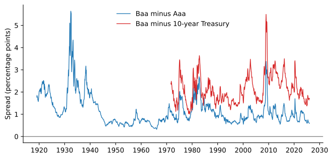
The Baa-Aaa spread averaged 1.16 percentage points from 1919 to 2025. It peaked at 5.64 points in May 1932, in the depths of the Great Depression, reached 3.38 points in December 2008, during the financial crisis, and was only 0.59 points at the end of 2025. The spread of Baa bonds over Treasuries averaged 2.12 points since 1971, with a peak of 5.5 points at the end of 2008. Spreads widen sharply in crises and recessions, when defaults are expected to rise and investors are least willing to bear risk, and narrow in good times.
Spreads are not just forecasts of defaults. Giesecke et al. (2011) assembled default rates on U.S. corporate bonds from 1866 to 2008. Default waves have been severe, and in the railroad crisis of 1873 to 1875 defaults amounted to 36% of the par value of the whole corporate bond market, far more than in the Great Depression. Default rates can be forecast with stock returns, stock market volatility and GDP growth, but surprisingly not with credit spreads, and spreads do not adjust to realized default rates. Over the long run, spreads have been about twice as large as default losses, which leaves a credit risk premium of about 80 basis points a year.
How Much of the Spread Is Default?
Elton et al. (2001) decomposed the spreads of investment-grade corporate bonds over Treasuries. For 10-year A-rated industrial bonds, expected default losses explain only 17.8% of the spread, and state and local taxes, which are paid on the whole coupon of a corporate bond, explain 36.1%. The remaining 46% behaves like a risk premium: up to 85% of it can be explained by the same Fama-French factors that price stocks.
A different approach starts from a model of default. Merton (1974) observed that the shareholders of a firm with debt hold a call option on its assets, with the face value of the debt as the strike: if the assets are worth less than the debt at maturity, they walk away. Bondholders hold the other side, a riskless bond minus a put option on the firm’s assets, and the yield spread is the value of that put. Huang and Huang (2012) calibrated this and several related structural models to historical default rates and to the equity premium. The models explain less than 20% of the spreads of investment-grade bonds, except for ten-year Baa bonds, but a much larger share of the spreads of high-yield bonds, a gap known as the credit spread puzzle. Chen et al. (2009) show that the puzzle shrinks once defaults and risk premia are allowed to rise together in recessions, as they do in a model that also matches the equity premium: a default in a bad state of the world costs investors more than one in a good state.
Credit default swaps offer a more direct measure. A credit default swap pays the buyer the loss on a bond if its issuer defaults, so its premium prices default risk alone. Comparing swap premia with bond spreads, Longstaff et al. (2005) find that the default component is the majority of the spread over Treasuries in every rating category: 51% for AAA and AA bonds, 56% for A, 71% for BBB and 83% for BB. The rest varies over time with measures of the illiquidity of individual bonds and of the bond market as a whole. The spread of an investment-grade bond therefore contains a large compensation for default risk, much more than the expected default loss, plus a liquidity premium and the effect of taxes.
Corporate Bond Returns
Corporate bonds trade over the counter, and until 2002 there was no public record of their prices. Since then, dealers have reported their trades to the Financial Industry Regulatory Authority through its TRACE system, and WRDS builds monthly bond returns from those transaction prices. We use these data for 115,769 non-convertible bonds with at least one year to maturity, and form value-weighted portfolios of investment-grade and high-yield bonds. Table 1 reports their excess returns over Treasury bills from September 2002 to December 2025.
| Mean (%) | Volatility (%) | Sharpe ratio | Worst month (%) | |
|---|---|---|---|---|
| Investment grade | 3.11 | 5.87 | 0.53 | -6.08 |
| High yield | 4.98 | 7.87 | 0.63 | -14.22 |
| All corporate bonds | 3.39 | 5.91 | 0.57 | -7.09 |
| Stock market | 10.37 | 15.18 | 0.68 | -17.20 |
Investment-grade bonds earned 3.1% a year over bills and high-yield bonds 5.0%, with volatilities well below that of stocks. Their Sharpe ratios were close to the stock market’s, in a period in which falling interest rates helped all bonds. Both had their worst month in March 2020, when the pandemic froze the corporate bond market, until the Federal Reserve announced that it would buy corporate bonds.
What risks do these returns compensate? Table 2 regresses the portfolios’ excess returns on the stock market factor MKT and on a Treasury factor TERM, the excess return of a 5-year zero-coupon Treasury from the yield curve of Bond Pricing.
| Alpha (%) | t(alpha) | MKT | TERM | R-squared | |
|---|---|---|---|---|---|
| Investment grade, CAPM | 1.42 | 1.10 | 0.16 | 0.18 | |
| Investment grade, MKT and TERM | -0.45 | -0.52 | 0.20 | 0.85 | 0.61 |
| High yield, CAPM | 1.14 | 0.73 | 0.37 | 0.51 | |
| High yield, MKT and TERM | 0.62 | 0.40 | 0.38 | 0.24 | 0.53 |
| All corporate bonds, CAPM | 1.30 | 1.04 | 0.20 | 0.27 | |
| All corporate bonds, MKT and TERM | -0.32 | -0.33 | 0.23 | 0.74 | 0.59 |
Investment-grade bonds behave mostly like Treasuries with a little equity risk. Their TERM loading is 0.85 and their MKT loading 0.20, and the two factors explain 61% of their variance. High-yield bonds behave more like stocks: their MKT loading is 0.38 and their TERM loading only 0.24, because the risk of default, which rises when the stock market falls, dominates their interest rate risk. Once both factors are included, none of the alphas is significant. The returns of corporate bonds look like compensation for interest rate risk and for the equity-like risk of default, consistent with the finding of Elton et al. (2001) that the part of the spread not explained by expected losses and taxes is related to the factors that price stocks.
Factor Models for Bonds
Fama and French (1993) built their three-factor model of Beyond the CAPM to price bonds as well as stocks. They added a term factor and a default factor, the return of long-term corporate bonds minus that of long-term Treasuries, and found that these two factors capture most of the variation in bond returns. More recent work asks whether characteristic-based factors, like those of the stock market, are needed to price corporate bonds. Bai et al. (2019) proposed factors based on downside risk, credit risk and liquidity risk and reported that they outperformed other models. The paper was retracted in 2023 after Dickerson et al. (2023) found that its result came from an error in the data, the misalignment in time of different series. With correctly aligned data, Dickerson, Mueller and Robotti find that a single factor, the return of the corporate bond market, is hard to beat, and that the proposed factors add little to it, except marginally for liquidity. The episode is a reminder of the replication problems of CAPM Anomalies and Beyond the CAPM: when returns are built from complex data, the alignment of the dates is part of the result.
Credit spreads also carry information about the economy. Collin-Dufresne et al. (2001) found that the variables that should explain changes in credit spreads, such as interest rates, leverage and volatility, explain little of them, and that the rest is driven mostly by a single common factor. Gilchrist and Zakrajšek (2012) split corporate spreads into the part explained by expected defaults and an excess bond premium, the price of bearing corporate credit risk beyond expected defaults. The excess bond premium rises when financial intermediaries lose capital, and it predicts declines in economic activity, consistent with a contraction in the supply of credit.
Reaching for Yield
Investors who want higher income can buy bonds with higher yields, but a higher promised yield is not a higher expected return if it comes with more default risk. Choi and Kronlund (2018) define reaching for yield as tilting a portfolio toward bonds with yields above those of its benchmark. Corporate bond mutual funds that reach for yield earn higher returns and attract more inflows, especially when interest rates are low, but their risk-adjusted returns tend to be negative. They also hold less cash and less liquid bonds, which makes them more vulnerable to redemptions. A fund that reaches for yield looks better than its benchmark in good times because it holds more credit risk, and the right benchmark, as in Performance Evaluation, is one with the same exposure to default risk.
Practice Problems
These problems give you a chance to practice the concepts introduced in this chapter. Try to solve each one on your own before expanding the solution.
Problem 1 (Promised and Expected Returns) Fenwick Industries has a one-year zero-coupon bond with a promised yield of 7%. One-year Treasuries yield 4%. The probability that Fenwick defaults within the year is 2%, and bondholders would recover 50% of the face value.
- Compute the bond’s expected return with (1).
- How much of the 3-point spread is expected default loss, and how much is expected excess return?
- A second issuer has the same spread but a default probability of 0.5% and the same recovery. How do the answers change?
Solution
1.07 \times (1 - 0.02 \times 0.5) - 1 = 5.93\%.
The expected loss is 7\% - 5.93\% = 1.07 points of the spread, and the expected excess return over Treasuries is 5.93\% - 4\% = 1.93 points.
The expected return is 1.07 \times (1 - 0.005 \times 0.5) - 1 = 6.73\%, so the expected loss is only 0.27 points and the expected excess return 2.73 points. With the same spread, a safer issuer leaves more of the spread as a premium.
Problem 2 (A Break-Even Default Rate) A five-year corporate bond yields 1.5 percentage points more than a Treasury of the same maturity. Recovery in default is 40% of face value.
- If the whole spread were compensation for expected default losses, what annual default probability would it imply?
- Historical default rates for bonds of this rating average about 0.3% a year. What share of the spread do expected losses explain? What else could explain the rest?
Solution
Approximately, the spread equals \pi (1 - R), so \pi = 0.015 / 0.6 = 2.5\% a year.
The expected loss is 0.003 \times 0.6 = 0.18 points, or 12% of the spread. The rest compensates for the systematic risk of default, which rises in recessions, for the bond’s illiquidity, and for the state taxes on corporate interest that Treasury investors do not pay.
Problem 3 (Debt as a Riskless Bond Minus a Put) A firm has assets worth $100 million and a single zero-coupon bond with a face value of $80 million due in one year. The risk-free rate is 5% a year with annual compounding, and a put option on the firm’s assets with a strike of $80 million and one year to maturity is worth $3 million.
- What are the values of the firm’s debt and equity?
- What is the promised yield of the debt and its spread over the risk-free rate?
- Why does the spread widen if the volatility of the firm’s assets rises?
Solution
The debt is worth a riskless bond minus the put, 80/1.05 - 3 = 76.19 - 3 = \$73.19 million, and the equity the rest, 100 - 73.19 = \$26.81 million.
The promised yield is 80/73.19 - 1 = 9.30\%, a spread of 4.30 percentage points over the 5% risk-free rate.
The put is worth more when the assets are more volatile, so the debt is worth less and its promised yield rises. The shareholders hold a call on the assets, which gains from the same volatility, so higher risk transfers value from bondholders to shareholders.
Problem 4 (Where Does a Bond Fund’s Return Come From?) A corporate bond fund has a TERM loading of 0.8, a MKT loading of 0.15 and an alpha of zero. Over a year, the excess return of the 5-year Treasury is -4\% and the stock market’s excess return is +10\%.
- What excess return does the model predict for the fund?
- A high-yield fund has a TERM loading of 0.25 and a MKT loading of 0.4. What does the model predict for it?
- Which fund would you expect to do better in a year in which stocks fall 20% and Treasury yields fall?
Solution
0.8 \times (-4\%) + 0.15 \times 10\% = -1.7\%.
0.25 \times (-4\%) + 0.4 \times 10\% = 3.0\%.
The investment-grade fund. Falling Treasury yields give positive TERM returns, which it holds mostly, while its small MKT loading limits its loss from the stock market. The high-yield fund loses more from the stock market decline and gains less from the fall in yields.