Skill versus Luck
The previous chapter measured the performance of one fund at a time. This chapter asks what the evidence says about active managers as a group. There are two questions. The first is whether active management pays on average: do the funds that try to beat the market, taken together, earn more than a passive index after their costs? The second is about individual managers. With thousands of funds in the data, some will have spectacular records even if no one has any skill, just as some coins in a large sample come up heads ten times in a row. Telling skill from luck in a large cross-section takes more than looking at the best records.
A third question sits behind both. Even if some managers have skill, competition among investors for those managers may leave nothing for the investors. Fund performance net of fees may be the wrong place to look for skill.
The Average Active Fund
Jensen (1968) found that mutual funds, on average, could not beat a buy-and-hold portfolio with the same beta, even before management expenses. Later studies with better data confirmed the result. Malkiel (1995) studied every diversified equity fund sold to the public from 1971 to 1991, including those that later disappeared, and recommended low-expense index funds. Gruber (1996) found that common stock funds underperformed the market by 1.94% a year from 1985 to 1994, and by 0.65% a year relative to a four-index model with the market, size, value and bond factors. Expense ratios in his sample averaged 1.13% a year, so before expenses the funds slightly beat their benchmarks. In his reading, active management adds value, but funds charge more than the value they add. Gruber’s question was why investors kept pouring money into actively managed funds when index funds were available.
Wermers (2000) used the quarterly holdings of funds to separate the stocks a fund holds from the fund’s net return. From 1975 to 1994, the stocks held by funds beat the market by 1.3% a year, but the funds’ net returns trailed it by 1%. Of the 2.3% difference, 0.7% came from the poor returns of the cash and bonds funds hold and 1.6% from expenses and transaction costs. Managers picked stocks well enough to cover their costs, but not well enough to leave anything for their investors.
What the Aggregate Fund Earns
The same pattern holds in recent data. The data for this chapter are the monthly returns of U.S. diversified equity funds in CRSP, January 1984 to December 2025. Share classes of the same fund are merged into one fund, and index funds and ETFs are excluded. The sample includes funds that later merged or closed, so it has no survivorship bias. It contains 5,181 active funds with at least $5 million in assets. Net returns are the returns investors receive. Gross returns add back one-twelfth of the expense ratio each month, so they are returns before fees but after trading costs.
| CAPM \alpha | t(\alpha) | Four-factor \alpha | t(\alpha) | |
|---|---|---|---|---|
| Value-weighted, net | -1.29 | -4.09 | -1.19 | -4.04 |
| Value-weighted, gross | -0.42 | -1.31 | -0.32 | -1.07 |
| Equal-weighted, net | -1.61 | -3.54 | -1.46 | -4.27 |
| Equal-weighted, gross | -0.46 | -1.00 | -0.30 | -0.88 |
Table 1 reports the alphas of the aggregate portfolio of all active funds. Net of costs, the value-weighted portfolio of active funds has a four-factor alpha of -1.19% a year, with a t-statistic of -4.04. Before fees, the alpha is -0.32% and statistically indistinguishable from zero. The difference between the two is roughly the average expense ratio, 0.88% a year. Fama and French (2010) found the same picture for 1984 to 2006: a value-weighted four-factor alpha of -1.00\% a year net and -0.05\% gross.
A gross alpha near zero is what simple arithmetic predicts. If index funds hold the market, the rest of the market is held by active investors, so the active investors as a group also hold the market. Before costs, their aggregate return is the market return, and after costs it is lower by exactly their costs. Mutual funds are only part of the active investors, so their gross alpha need not be zero exactly, but there is no reason for it to be far from zero. Active management as a whole is a zero-sum game before costs and a negative-sum game after them. This does not say that no manager is skilled. It says that the gains of skilled managers come at the expense of other active investors, and the question is whether we can find the winners in advance.
Survivorship Bias
A database that contains only the funds that exist today overstates past performance, because funds that did badly tend to be merged into other funds or closed. Malkiel (1995) found that from 1982 to 1991 the surviving funds earned 17.09% a year while all funds, including those that disappeared, earned 15.69%. Elton et al. (1996) measured the bias on alphas instead of raw returns. Following 188 funds from 1977 to 1993, they found that the merged funds had alphas of about -2.9\% a year before they disappeared, and that using only survivors overstates the average alpha by about 0.9% a year. The bias grows with the length of the study, because more funds disappear over longer periods: it was about 0.4% a year in a 10-year study and about 1% in a 20-year study.
Our sample shows the same effect. Of the funds with at least eight months of returns, 2,440 were still reporting in December 2025 and 3,639 had disappeared. The surviving funds have an average net four-factor alpha of -1.41% a year, while the funds that disappeared averaged -2.26%. A study that looked only at today’s funds would report an average alpha of -1.41% instead of -1.92%.
Brown et al. (1992) pointed to a subtler effect. If managers differ in how much risk they take, survivorship can create the appearance of persistent performance even when no one has skill. High-risk funds have extreme returns in both directions. Those that do badly are dropped from the sample, and those that do well survive, so among survivors the high-risk funds look like repeat winners. Studies of persistence must therefore use samples that include dead funds.
Does Performance Persist?
If some managers are skilled, the funds that did well in the past should keep doing well. Early evidence seemed to show this. Malkiel (1995) found that in the 1970s, funds with above-median returns in one year were above the median again the next year almost two-thirds of the time, but in the 1980s the winners repeated just over half the time. Persistence in his data was weaker in the decade with better data.
Carhart (1997) gave the classic answer. He sorted all diversified equity funds each year from 1962 to 1993 into deciles by their return over the previous year and followed each decile over the next year. The top decile beat the bottom decile by about 8% a year. Of that spread, 4.6% came from the size, value and especially the momentum exposure of the stocks the funds held, 0.7% from differences in expense ratios and 1% from transaction costs. Funds with the best past returns had ridden last year’s winning stocks, often by accident. Once momentum and costs are accounted for, there was no evidence of persistent skill. The only persistence that remained was among the worst funds, which continued to do badly.
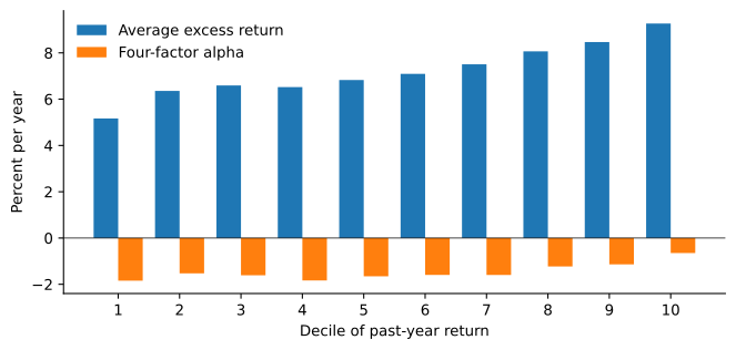
Figure 1 repeats Carhart’s sort on our sample. Last year’s winners again earn more than last year’s losers: the top decile beats the bottom one by 4.1% a year. The four-factor regression, though, gives the spread a momentum loading of 0.42 and an alpha of only 1.2% a year, with a t-statistic of 0.72. Every decile has a negative net alpha. Past winners hold stocks that went up, which keep going up for a while, and that is all.
Skill or Luck in a Large Cross-Section
Suppose no manager has any skill, so every fund’s true alpha is zero. The previous chapter showed that the t-statistic of a fund’s alpha is roughly its information ratio times the square root of the number of years (see How Precise Is a Measured Alpha?). With true alpha zero, each t-statistic is approximately standard normal, and a fund has a 2.3% chance of a t-statistic above 2 by luck alone. In a sample of thousands of funds, many will clear that bar.
Example 1 (Counting Lucky Funds) A database holds 4,000 funds, none of which has any skill. Their alpha t-statistics are independent standard normals.
The probability that one fund has t > 2 is 1 - \Phi(2) = 0.0228, so about 4{,}000 \times 0.0228 = 91 funds will show alphas that are “significant” at the usual level. The probability that a given fund has t > 3 is 0.00135, so the expected number of such funds is 5.4, and the probability that at least one fund has t > 3 is 1 - (1 - 0.00135)^{4{,}000} = 0.995. A single fund with t > 3 would be impressive. In a database of 4,000 funds it is almost certain to appear.
The right question is not whether the best funds have large t-statistics but whether there are more large t-statistics than luck would produce. Comparing with the normal distribution is not enough, though. Fund returns are not normal, funds have different numbers of observations, and fund returns are correlated with each other because funds hold similar stocks. The solution is to simulate the distribution of t-statistics under no skill, using the funds’ own returns.
Bootstrapping the Cross-Section
Kosowski et al. (2006) bootstrapped the four-factor regression of each fund separately. For each fund, they set the alpha to zero, resampled the regression residuals, and re-estimated the alpha, which shows how large the fund’s alpha could be by luck. In 1,788 funds with at least five years of returns, from 1975 to 2002, luck alone would produce nine funds with net alphas above 10% a year. In the data, 29 funds exceeded that level. They concluded that the stars among growth funds had genuine stock-picking talent, though such funds became scarcer after 1990.
Fama and French (2010) changed two things. First, they resampled calendar months rather than residuals, drawing the same months for all funds at once. This keeps the correlation of returns across funds, which matters because funds that hold similar stocks are lucky or unlucky together. Second, they required only eight months of returns, because a five-year minimum keeps only the funds that survived five years. The procedure is simple. Subtract each fund’s estimated alpha from its returns, so that every fund has a true alpha of zero. Draw a sample of months with replacement, re-estimate every fund’s alpha and its t-statistic on those months, and record the percentiles of the cross-section of t-statistics. Repeat many times. Each run is a world in which no manager has skill, and the simulated percentiles show what luck produces.
| Net actual | Net luck | Net below | Gross actual | Gross luck | Gross below | |
|---|---|---|---|---|---|---|
| 1st | -3.90 | -2.45 | 0 | -3.10 | -2.48 | 2 |
| 5th | -3.05 | -1.68 | 0 | -2.39 | -1.69 | 1 |
| 10th | -2.61 | -1.30 | 0 | -1.98 | -1.30 | 0 |
| 25th | -1.89 | -0.68 | 0 | -1.22 | -0.67 | 0 |
| 50th | -1.09 | 0.01 | 0 | -0.34 | 0.01 | 4 |
| 75th | -0.28 | 0.69 | 0 | 0.50 | 0.70 | 17 |
| 90th | 0.50 | 1.32 | 0 | 1.32 | 1.34 | 51 |
| 95th | 0.98 | 1.72 | 0 | 1.79 | 1.73 | 63 |
| 98th | 1.55 | 2.19 | 0 | 2.37 | 2.19 | 79 |
| 99th | 1.98 | 2.54 | 0 | 2.71 | 2.52 | 78 |
Table 2 applies the procedure to our sample, with 1,000 runs. For net returns, every percentile of the actual distribution is far below the one luck produces. Even the 99th percentile of the actual t-statistics, 1.98, is below the luck value of 2.54 in essentially every run. In net returns, a fund whose alpha looks large is no more than lucky, and most funds have negative true alphas. Gross returns tell a different story. The left tail is much worse than luck, so there are managers whose trading loses money even before fees. The right tail is close to what luck produces: the 98th percentile is 2.37 against 2.19 under no skill, and the simulated value is below the actual one in 79% of the runs. That is a hint of skill in the right tail, not strong evidence.
Fama and French (2010) reached similar conclusions. For net returns, “the simulation results are disheartening”: the true net alpha is negative for most if not all active funds. For gross returns, they found evidence of skill in both tails, inferior as well as superior managers. They estimated that if true gross alphas are normal with mean zero, a standard deviation of about 1.25% a year fits the tails of the data. That is not much skill: only about one fund in six would have a true alpha above 1.25% a year, before fees that take about 1% a year.
False Discoveries
Barras et al. (2010) asked a different question: what fraction of funds have zero, positive or negative true alphas? The tool is the false discovery rate from multiple testing in statistics. Each fund’s alpha has a p-value, the probability of a t-statistic as extreme as the one observed if the true alpha is zero. For funds whose true alpha is zero, p-values are uniformly distributed between 0 and 1. Funds with nonzero alpha tend to have small p-values, so large p-values come almost entirely from zero-alpha funds. If \pi_{0} is the fraction of zero-alpha funds among M funds, the number of p-values above some \lambda (say 0.5) should be about \pi_{0} M (1 - \lambda), which gives an estimate of \pi_{0}. Among the funds that are significant at level \gamma with a positive t-statistic, about \pi_{0} M \gamma / 2 are zero-alpha funds that got lucky. Subtracting them gives the fraction of skilled funds: \hat{\pi}_{0} = \frac{\#\{p_{i} > \lambda\}}{M (1 - \lambda)} \qquad \hat{\pi}^{+} = \frac{\#\{p_{i} < \gamma, \ t_{i} > 0\}}{M} - \hat{\pi}_{0} \frac{\gamma}{2}. \tag{1} The fraction of unskilled funds \hat{\pi}^{-} is estimated the same way from the significant negative t-statistics.
For 2,076 funds from 1975 to 2006, Barras et al. (2010) estimated that 75.4% of funds had zero alpha net of costs, 24.0% were unskilled and only 0.6% were skilled, a proportion statistically indistinguishable from zero. The fraction of skilled funds fell from 14.4% in 1990 to 0.6% in 2006, while the fraction of unskilled funds rose. Before expenses, 9.6% of funds were skilled. A zero-alpha fund is not one whose manager lacks skill. It is one whose manager has enough skill to cover costs and fees but not more.
Applying (1) with \lambda = 0.5 and \gamma = 0.2 to our sample, using the regression p-values of each fund’s four-factor alpha, gives a zero-alpha fraction of 57% in net returns, with 38% of funds unskilled and an estimated skilled fraction of zero. In gross returns the zero-alpha fraction rises to 79%, 15% are unskilled and 2% are skilled. The sample runs twenty years past theirs, and the drift they found continues: net of fees, skilled funds have become impossible to detect.
Harvey and Liu (2018) take yet another approach. Rather than testing each fund against zero, they estimate the cross-sectional distribution of true alphas and use it to shrink each fund’s estimated alpha toward the population. A fund with a large estimated alpha is more likely to be a fund with a modest true alpha and a lucky draw than a fund with a large true alpha, because large true alphas are rare. Shrinking reduces the error in forecasting future alphas, and the distribution it implies has a thin right tail. As they put it, past fund performance does a poor job of predicting future outcomes, and the reason is noise.
Skill in Equilibrium
The evidence so far seems to say that active managers lack skill. Berk and Green (2004) showed that the same evidence is consistent with a world in which most managers are skilled. Their model has three ingredients. Managers differ in ability, and each manager’s alpha before costs declines as the fund grows, because a larger fund must trade larger positions and move prices against itself. Investors learn about a manager’s ability from past returns. And investors supply capital competitively, moving money to any fund with a positive expected net alpha.
Money then flows into a fund with a good record until its expected net alpha falls to zero. If \alpha(q) is the gross alpha of a fund of size q and f its fee, the fund reaches the size q^{*} at which \alpha(q^{*}) - f = 0 \qquad \text{value added} = q^{*} \alpha(q^{*}) = q^{*} f. \tag{2} In equilibrium, investors in every fund expect a net alpha of zero, and all the value the manager creates goes to the manager as fees. Past performance does not predict future net returns, because good past performance attracts money until the expected net return is competitive again. A lack of persistence, or a zero average net alpha, is exactly what this model predicts, even with skilled managers. The model is partial equilibrium: it takes the returns available to managers as given.
The model needs flows that chase performance, and they do. Sirri and Tufano (1998) found that from 1971 to 1990, money flowed disproportionately into the funds with the best recent returns, while investors did not leave the worst funds at the same rate.
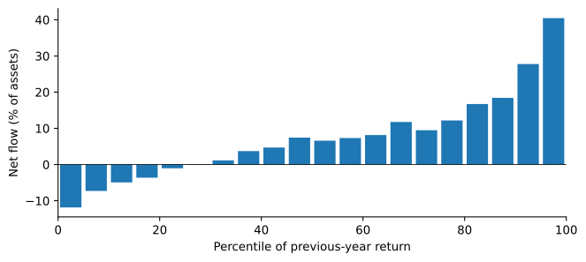
Figure 2 shows the relation in our sample, 1992 to 2025. Funds in the top 5% of last year’s returns grow by 40% of their assets through new money, and funds in the next 5% by 28%, while funds in the bottom 5% shrink by only 12%. Flows chase performance, and much more strongly for winners than losers.
Fama and French (2010) disagreed with the Berk and Green interpretation. In the model, funds with positive alphas before costs grow until their net alphas are zero, so the average net alpha should be zero. But the average net alpha is negative, and the bootstrap shows that most funds have negative net alphas. Their verdict was that the model is attractive theory, but the data reject most of its predictions about fund returns.
Berk and Binsbergen (2015) argued that net alpha is the wrong measure of skill. A manager’s skill shows up in the total dollars the fund extracts from the market, gross of fees, which they call value added: the fund’s gross return in excess of a benchmark, multiplied by its assets. They used as benchmarks the net returns of Vanguard index funds, which investors could actually have bought. From 1977 to 2011, the average fund added about $3.2 million a year (in 2000 dollars), though the median fund lost value. Cross-sectional differences in value added persisted for as long as ten years, and investors rewarded skill by giving more money to the funds with more value added. In their reading, managers have skill, and they capture its value as fees.
Table 3 repeats their calculation in our sample, split at 2011, the end of their sample. For each fund with at least 36 months in a period, value added is the average over its months of the lagged assets, in 2025 dollars, times the gross return in excess of a benchmark of the same four-factor exposures. Following Berk and van Binsbergen, the weighted mean weights each fund by its number of months, so it is the value added by the average fund-month. Their $3.2 million in 2000 dollars is about $6.1 million in 2025 dollars.
| Funds | Weighted mean | t, funds | t, months | Median | Positive (%) | |
|---|---|---|---|---|---|---|
| 1984 to 2011 | 3211 | 9.48 | 4.34 | 0.79 | -0.39 | 45 |
| 2012 to 2025 | 2673 | -10.49 | -3.55 | -1.05 | -3.34 | 17 |
Through 2011 the weighted mean is 9.48 million dollars a year, even larger than theirs, while the median fund lost 0.39 million and only 45% of funds added value. Since 2012 the average fund-month has lost 10.49 million a year, and only 17% of funds added value.
How precise are these averages? Berk and van Binsbergen compute the standard error across funds. Each fund’s average monthly value added is one observation, and the standard error of the weighted mean treats the roughly 6,000 fund averages as independent draws, which gives them a t-statistic of 5.74. The first t-statistic in Table 3 repeats this calculation. Treating funds as independent, both of our averages also look highly significant, with t-statistics of 4.34 and -3.55.
But funds are not independent. In any month, funds tend to win or lose together, because they share exposures that the benchmark leaves out. The second t-statistic accounts for this. It averages value added across funds in each month, weighting each month by its number of funds so that the mean of the series is the same fund-month average, and computes the standard error from this monthly series, with Newey-West standard errors over six lags. A shock common to all funds then moves one monthly observation instead of counting as thousands of independent ones. With this correction, the t-statistics fall to 0.79 and -1.05. Neither period’s value added is distinguishable from zero.
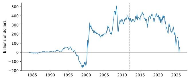
Figure 3 adds up the value added of all funds month by month. The total is dominated by a few years. In 2000, when the technology bubble burst, active funds beat their benchmarks by 465 billion dollars before fees, more than their entire cumulative value added through 2011. Without that one year, the total through 2011 is negative. The losses since 2012 are concentrated in the same way, in 2016 and 2024. Value added measured in dollars rests on a handful of episodes in which most funds won or lost together, which is exactly when treating funds as independent overstates the evidence. Berk and van Binsbergen acknowledge that correlation across funds overstates their t-statistic, and they rest their case on persistence instead: funds ranked in the top decile by past value added keep beating those in the bottom decile, in tests that average over funds each month, as our second t-statistic does. The level of value added, though, is not distinguishable from zero in either period.
Pástor et al. (2015) asked whether the decreasing returns to scale in the model come from the size of each fund or from the size of the whole industry. A fund’s alpha may fall when the fund grows, or when the industry grows, because more money chases the same mispricings. They found that fund-level decreasing returns are hard to measure precisely, while industry-level decreasing returns are strong: a 1 percentage point increase in the active fund industry’s share of the stock market reduces a typical fund’s performance by about 0.03% a month, almost 0.4% a year. Their estimates of skill rose over time, from 0.24% a month in 1979 to 0.42% in 2011, while performance stayed flat. Managers became more skilled, but the industry grew, and the competition among more active dollars for the same opportunities offset the gain.
Looking Inside the Portfolio
Return-based tests treat a fund as a black box. Holdings data let us look inside. Wermers (2000), discussed above, used holdings to separate stock-picking from costs. Two further measures from holdings have attracted attention.
Cremers and Petajisto (2009) measure how different a fund’s holdings are from its benchmark index. If w_{i} is the fund’s weight in stock i and w^{B}_{i} the benchmark’s weight, the fund’s active share is A fund that holds the index has an active share of zero, and a fund with no stocks in common with the index has an active share of one. They found that funds with the highest active share beat their benchmarks by 1.13 to 1.15% a year after fees, while the funds with the lowest active share, closet indexers that charge active fees for passive portfolios, underperformed. Closet indexing grew from almost nothing in the 1980s to about 30% of fund assets in 2003. Frazzini et al. (2016) used the same data and found that the result comes from the benchmarks. High-active-share funds tend to have small-cap benchmarks, so sorting on active share amounts to sorting on benchmark, and most of the outperformance of high-active-share funds reflects the poor risk-adjusted returns of their benchmarks rather than good returns of the funds. Comparing funds with the same benchmark, active share was as likely to predict performance positively as negatively. Active share measures how much of the fee buys active management, but not whether that management is good.
Kacperczyk et al. (2008) compared a fund’s return with the return of its most recently disclosed holdings, net of expenses. The difference, the return gap, captures what the fund does between disclosures: trades that add value, as well as trading costs and other hidden costs. The return gap persists for up to five years, and funds with the largest past return gaps beat those with the smallest by about 3.4% a year.
Hedge Funds
Hedge funds are harder to evaluate than mutual funds, for three reasons. Their strategies change exposures quickly and use derivatives and leverage, so factor models built from stock portfolios fit them poorly. Many hold illiquid assets whose prices are estimates. And they are not required to report returns to anyone, so the databases contain only the funds that choose to report.
Dynamic Strategies and Their Benchmarks
Fung and Hsieh (1997) ran the returns of mutual funds and hedge funds on the returns of eight asset classes. For mutual funds, the asset classes explained most of the variance: 47% of funds had an R^{2} above 75%. For hedge funds, nearly half had an R^{2} below 25%, and a quarter were negatively correlated with the asset classes. Hedge fund returns were not driven by what they held but by how they traded. Trend-following funds, for example, had returns that looked like a straddle on U.S. equities: they did well in large market moves in either direction.
Fung and Hsieh (2004) built benchmarks from this insight. Their seven factors include the stock market, a small-minus-large stock factor, changes in the ten-year Treasury yield and in the credit spread, and the returns of lookback straddles on bonds, currencies and commodities, which mimic trend-following strategies. Over 1994 to 2002, these factors explained about half of the variance of an index of funds of hedge funds. The full-sample alpha was a significant 0.48% a month, but in the subperiods between structural breaks in the factor exposures the alphas were small and insignificant. They called it an “alpha illusion”: much of what looked like alpha was compensation for exposures to option-like risks.
Stale Prices and Smoothed Returns
When a fund holds assets that trade rarely, its reported value at the end of a month uses stale or estimated prices. A market decline shows up in the fund’s reported return only gradually, over several months. Asness et al. (2001) found that the monthly returns of a broad hedge fund index from 1994 to 2000 had a beta of only 0.37 on the S&P 500. Adding the market returns of the three previous months to the regression and summing the betas raised the beta to 0.84. The annual alpha fell from 2.6% to about -4.5\%, which was not significantly different from zero.
Getmansky et al. (2004) modeled this effect. Suppose the fund’s true return R_{t} is serially uncorrelated, but the reported return is a weighted average of the current and past true returns: R^{o}_{t} = \theta_{0} R_{t} + \theta_{1} R_{t - 1} + \cdots + \theta_{k} R_{t - k} \qquad \theta_{j} \geq 0 \qquad \theta_{0} + \theta_{1} + \cdots + \theta_{k} = 1. \tag{4} The weights sum to one, so the reported returns have the same mean as the true returns. Their variance is smaller, though, by the factor \theta_{0}^{2} + \cdots + \theta_{k}^{2} < 1, so the reported Sharpe ratio is too high: \sigma(R^{o}) = \sigma(R) \sqrt{\theta_{0}^{2} + \cdots + \theta_{k}^{2}} \qquad \text{SR}^{o} = \frac{\text{SR}}{\sqrt{\theta_{0}^{2} + \cdots + \theta_{k}^{2}}}. \tag{5} The beta on the current market return is \theta_{0} \beta, biased toward zero, and the true beta \beta is recovered by summing the betas on the current and lagged market returns. Smoothing also makes reported returns serially correlated. Getmansky, Lo and Makarov found the strongest smoothing in fund categories that hold illiquid assets, such as fixed-income and convertible bond funds. Their main interpretation was illiquidity, not deliberate manipulation, though smoothing has the same effect on the numbers either way.
Example 2 (A Smoothed Fund) A fund’s true monthly returns have an annualized Sharpe ratio of 0.5 and a market beta of 0.8, but it reports returns smoothed with weights \theta_{0} = 0.5, \theta_{1} = 0.3 and \theta_{2} = 0.2.
The sum of squared weights is 0.25 + 0.09 + 0.04 = 0.38, so the reported volatility is \sqrt{0.38} = 0.62 times the true volatility and the reported Sharpe ratio is 0.5 / 0.62 = 0.81. The beta on the current market return is 0.5 \times 0.8 = 0.4, half the true beta, and regressing on the current and two lagged market returns gives betas of 0.4, 0.24 and 0.16, which sum to 0.8. The first-order autocorrelation of reported returns is (\theta_{0} \theta_{1} + \theta_{1} \theta_{2}) / 0.38 = 0.21 / 0.38 = 0.55. An investor who used the reported returns would think the fund was a low-beta fund with a Sharpe ratio well above the market’s.
Reporting Biases
Hedge funds report returns to commercial databases voluntarily, and they can stop reporting when they choose. Aiken et al. (2013) found a way around this. Funds of hedge funds registered with the SEC must disclose their holdings, including the value of each hedge fund they hold, so these filings reveal the returns of hedge funds whether or not they report to a database. From 2004 to 2009, funds that reported to a database had a seven-factor alpha of 1.20% a quarter, while funds that did not report had an alpha of 0.05% a quarter, statistically zero. Funds that stopped reporting did badly after they stopped. Databases contain the funds that have good news to share.
Bollen and Pool (2009) looked at the distribution of reported monthly returns. Across hedge funds, small gains are far more common than small losses: the distribution has a kink at zero. The kink disappears in two-month returns and in the months around audits, which suggests that some managers report small losses as small gains and correct them later. Bollen and Pool concluded that the kink is caused at least in part by temporarily overstated returns, while noting that optimistic valuations of illiquid holdings could also produce it.
Skill and What Investors Earn
Despite these problems, the evidence for skill among hedge funds is stronger than among mutual funds. Kosowski et al. (2007) applied the bootstrap of Kosowski et al. (2006) to hedge funds from 1994 to 2002, measured against the seven factors of Fung and Hsieh (2004). By luck alone, at most three funds would have alpha t-statistics of at least 4.67, but 155 funds did. Persistence was mild when funds were sorted on estimated alphas, but strong when the alphas were estimated with Bayesian methods that pool information across funds. Jagannathan et al. (2010) found that about a quarter to a third of a hedge fund’s alpha relative to its style index carries over into the next three years. The persistence is among the top funds, with little among the worst.
What investors earn is another matter. Dichev and Yu (2011) computed the dollar-weighted returns of hedge fund investors, as in the previous chapter’s comparison of time- and dollar-weighted returns. From 1980 to 2008, the aggregate buy-and-hold return of hedge funds was 12.6% a year, but the dollar-weighted return was only 6.0%, below the S&P 500’s 10.9% and barely above the risk-free rate of 5.6%. Investors put money in after good returns, so the most money was invested just before the bad years, 2008 above all. By their estimate, the timing cost was large enough that the alpha hedge fund investors actually earned was close to zero.
What the Evidence Says
The average active mutual fund loses to an index fund by roughly its fees, as the arithmetic of active management predicts. Past winners keep winning only in the sense that their stocks have momentum. In a large cross-section, the best records in net returns are what luck would produce. In gross returns there is evidence of skill in both tails, but the right tail is thin. The equilibrium view of Berk and Green reconciles these facts with skilled managers: competition for skill drives investors’ net alphas to zero, and managers collect the value they create as fees. Hedge funds offer more evidence of skill, but their data are harder to trust, and their investors have earned much less than the funds themselves.
For an investor, the practical conclusion is the one Malkiel (1995) drew three decades ago: a low-cost index fund is hard to beat. For a student of markets, the conclusion is more interesting. Prices are close enough to efficient that skill is scarce and expensive, but not so efficient that skill earns nothing.
Practice Problems
These problems give you a chance to practice the concepts introduced in this chapter. Try to solve each one on your own before expanding the solution.
Problem 1 (The Arithmetic of Active Management) Index funds hold 45% of a stock market, and active investors hold the rest. The market returns 9\% in a year. Index funds charge 0.05\%, and active investors pay 0.85\% in fees and 0.25\% in trading costs.
- What is the return of the aggregate portfolio of active investors before costs?
- What do index fund investors and active investors earn as groups after costs?
- Does this mean that no active manager can beat the market?
Solution
The market is the sum of the index funds’ holdings and the active investors’ holdings. The index funds hold the market portfolio, so the active investors together also hold the market portfolio, and their aggregate return before costs is 9\%.
Index fund investors earn 9 - 0.05 = 8.95\%. Active investors as a group earn 9 - 0.85 - 0.25 = 7.90\%.
No. The argument is about the average dollar invested actively. Some active managers beat the market, but only at the expense of other active investors who trail it by the same amount before costs. The question for an investor is whether the winners can be identified in advance.
Problem 2 (Survivorship Bias) A database tracks 500 funds from 2005 to 2025. By 2025, 150 funds have merged or closed; while they existed they had an average alpha of -3.0\% a year. The 350 survivors have an average alpha of -0.6\% a year.
- What average alpha would a study that uses only the surviving funds report?
- What is the average alpha of all 500 funds, with each fund weighted equally?
- What is the survivorship bias? Why would it be larger in a 30-year study?
Solution
A study of the survivors reports -0.6\% a year.
The average of all funds is 0.7 \times (-0.6) + 0.3 \times (-3.0) = -0.42 - 0.90 = -1.32\% a year.
The bias is -0.6 - (-1.32) = 0.72 percentage points a year. Over a longer study more funds disappear, and the funds that disappear are mostly poor performers, so the gap between the survivors and the full sample grows.
Problem 3 (Winners and Losers) A study ranks 400 funds by their returns in two consecutive three-year periods. A fund is a winner in a period if its return is above the median. The counts are: 120 winners in both periods (WW), 80 winners then losers (WL), 80 losers then winners (LW) and 120 losers in both periods (LL). The cross-product ratio and the standard error of its logarithm are \text{CPR} = \frac{\text{WW} \times \text{LL}}{\text{WL} \times \text{LW}} \qquad \text{se}(\ln \text{CPR}) = \sqrt{\frac{1}{\text{WW}} + \frac{1}{\text{WL}} + \frac{1}{\text{LW}} + \frac{1}{\text{LL}}}.
- Compute the cross-product ratio. What value would it have with no persistence?
- Test whether the persistence is statistically significant.
- Give two reasons why this persistence need not mean that managers are skilled.
Solution
\text{CPR} = (120 \times 120) / (80 \times 80) = 2.25. With no persistence, a winner is as likely as a loser to win in the next period, so all four counts are equal and the ratio is 1.
\ln 2.25 = 0.811 and \text{se} = \sqrt{2 / 120 + 2 / 80} = \sqrt{0.0417} = 0.204, so z = 0.811 / 0.204 = 3.97. The persistence is significant.
First, the persistence may come from the stocks the funds hold rather than from skill: funds that held last year’s winners keep riding their momentum, and funds with high expenses keep losing to those with low expenses. Second, if the sample keeps only funds that survived both periods and funds differ in risk, survivorship alone produces persistence. It is also worth checking whether the persistence comes from winners repeating or from losers repeating, which is the more common finding.
Problem 4 (A Fund in Equilibrium) A manager’s gross alpha falls with the size of the fund, \alpha(q) = 3\% - 0.5\% \times q, where q is the fund’s assets in billions of dollars. Investors move money in and out of the fund until its expected net alpha is zero.
- If the fee is 1\% a year, how large does the fund become? What do its investors earn, and how much value does the manager add each year?
- If the manager raises the fee to 1.5\%, how large does the fund become, and what are the manager’s fee revenues?
- What fee maximizes the manager’s revenues? Does the fee affect what investors earn?
Solution
By (2), 3 - 0.5 q = 1, so q^{*} = 4 billion dollars. Investors earn a net alpha of zero. The value added is q^{*} \alpha(q^{*}) = 4 \times 1\% = \$40 million a year, all of which the manager collects as fees.
Now 3 - 0.5 q = 1.5, so q^{*} = 3 billion dollars, and fee revenues are 3 \times 1.5\% = \$45 million a year.
With a fee of f percent, the fund grows to q = (3 - f) / 0.5 = 2 (3 - f) billion dollars, and revenues are 10 f q = 20 f (3 - f) million dollars. This is maximized at f = 1.5\%, the fee of part (b). Whatever the fee, investors earn a net alpha of zero: the fee decides the size of the fund and how much the manager earns, not what investors get.
Problem 5 (Reading Smoothed Returns) A hedge fund’s true monthly returns are serially uncorrelated, with an annualized Sharpe ratio of 0.6 and a market beta of 0.5. The fund reports smoothed returns as in (4), with \theta_{0} = 0.6, \theta_{1} = 0.3 and \theta_{2} = 0.1.
- What Sharpe ratio does an analyst compute from the reported monthly returns?
- What beta does a regression of reported returns on the current market return give?
- What is the first-order autocorrelation of reported returns?
- How can the analyst recover the true beta?
Solution
The sum of squared weights is 0.36 + 0.09 + 0.01 = 0.46, and \sqrt{0.46} = 0.678. By (5) the reported Sharpe ratio is 0.6 / 0.678 = 0.88.
The beta on the current market return is \theta_{0} \beta = 0.6 \times 0.5 = 0.30.
The covariance of R^{o}_{t} and R^{o}_{t - 1} is (\theta_{0} \theta_{1} + \theta_{1} \theta_{2}) \sigma^{2}, so the autocorrelation is (0.18 + 0.03) / 0.46 = 0.46.
Regress the reported returns on the current and two lagged market returns. The slopes are \theta_{0} \beta = 0.30, \theta_{1} \beta = 0.15 and \theta_{2} \beta = 0.05, and their sum is the true beta, 0.5.
Problem 6 (How Many Funds Are Skilled?) An analyst estimates four-factor alphas for 2,000 funds. Of their p-values, 700 are above 0.5. At a significance level of 0.10, 180 funds have significant positive alphas and 260 have significant negative alphas.
- Estimate the fraction \pi_{0} of funds with zero true alpha.
- How many of the 180 significant positive alphas are expected to be zero-alpha funds that were lucky?
- Estimate the fractions of skilled and unskilled funds.
- The three fractions do not add up to one. Why not?
Solution
By (1), \hat{\pi}_{0} = 700 / (2{,}000 \times 0.5) = 0.70.
Zero-alpha funds have uniformly distributed p-values, so a fraction 0.10 / 2 = 0.05 of them have significant positive alphas: 0.70 \times 2{,}000 \times 0.05 = 70 funds.
Skilled: (180 - 70) / 2{,}000 = 5.5\%. Unskilled: (260 - 70) / 2{,}000 = 9.5\%.
The three fractions add up to 85\%. The remaining 15\% are funds with nonzero true alphas that are too small, or measured too imprecisely, to be significant at the 0.10 level. Using a larger significance level counts more of them.