The Treynor-Black Model

Most investors cannot analyze every security. A research department covers a few dozen stocks at most, and for the thousands of others the best guess is that the market prices them fairly. Treynor and Black (1973) showed how such an investor should use the analysts’ work. Hold the market portfolio, which needs no forecasts, and add an active portfolio of the securities the analysts believe are mispriced, sized according to how good the forecasts are. The model rests on the single-index model of The Index Model, which keeps the inputs manageable: an alpha, a beta and a residual variance for each analyzed security, and the expected return and variance of the market.

Model Setup

We have N risky assets with excess returns following a single-index model R_{i} = \alpha_{i} + \beta_{i} R_{M} + e_{i}, where \operatorname{E}(e_{i}) = 0, \operatorname{Cov}(R_{M}, e_{i}) = 0 and \operatorname{Cov}(e_{i}, e_{j}) = 0 for i \neq j, for all i, j = 1, \ldots, N. Suppose we form a portfolio P with the N risky assets and the market portfolio M.

Denote by w_{i} the weights of the N risky assets and w_{M} the weight in the market portfolio. Of course, the sum of the portfolio weights must be equal to one, i.e., \sum_{i = 1}^{N} w_{i} + w_{M} = 1. \tag{1}

We can write the excess returns of this portfolio over the risk-free asset as R_{P} = \alpha_{P} + \beta_{P} R_{M} + e_{P}. The portfolio alpha includes the alpha of all the securities except the market, which has no alpha, and the beta of the portfolio is a weighted average of the betas of all securities and the beta of the market, which is one: \alpha_{P} = \sum_{i = 1}^{N} w_{i} \alpha_{i}, \qquad \beta_{P} = \sum_{i = 1}^{N} w_{i} \beta_{i} + w_{M}. \tag{2} We will see later that the alpha of the optimal portfolio is positive, since its weights are positive for securities with positive alpha and negative otherwise. Choosing w_{M} given the weights of the other assets is the same as choosing \beta_{P}, so we will choose the weights in the individual assets and the beta of the portfolio.

The idiosyncratic risk includes the firm-specific risks of all securities except the market, which has none. Because the firm-specific risks are uncorrelated with each other, we have that \sigma^{2}(e_{P}) = \sum_{i = 1}^{N} w_{i}^{2} \sigma^{2}(e_{i}). \tag{3} Thus, \operatorname{E}(R_{P}) = \sum_{i = 1}^{N} w_{i} \alpha_{i} + \beta_{P} \operatorname{E}(R_{M}), \qquad \sigma_{P}^{2} = \beta_{P}^{2} \sigma_{M}^{2} + \sum_{i = 1}^{N} w_{i}^{2} \sigma^{2}(e_{i}). \tag{4} The expected return and variance in (4) depend on the alphas generated by the active securities and the systematic exposure of the resulting portfolio. This is the essence of the Treynor-Black model. The active part of the portfolio generates an alpha but adds diversifiable risk. It may also change the portfolio’s beta, and with it the systematic risk and the expected return that comes with it.

Solving the Model

The objective is to find the portfolio weights w_{1}, w_{2}, \ldots, w_{N} and w_{M} that maximize its Sharpe ratio, which is equivalent to finding w_{1}, w_{2}, \ldots, w_{N} and the beta of the portfolio.

Maximizing the Sharpe ratio is equivalent to minimizing the variance of the portfolio for a given expected return. Only one particular expected return satisfies the restriction in (1). For other targets of the expected return, we would have to borrow or invest the difference at the risk-free rate. If we denote by \mu_{P} a possible target expected return, the minimization problem is \min_{\{w_{1}, w_{2}, \ldots, w_{N}, \beta_{P}\}} \; \frac{1}{2} \sigma_{P}^{2} \quad \textrm{s.t.} \quad \operatorname{E}(R_{P}) = \mu_{P} - r_{f}. With a Lagrange multiplier \lambda, the first-order conditions for the weights and the beta are w_{i} \sigma^{2}(e_{i}) - \lambda \alpha_{i} = 0, \quad i = 1, \ldots, N, \qquad \beta_{P} \sigma_{M}^{2} - \lambda \operatorname{E}(R_{M}) = 0. The condition on the expected return is not important, since we will compute \lambda later by imposing that the weights add up to one. The first condition implies that for each security w_{i} = \lambda \frac{\alpha_{i}}{\sigma^{2}(e_{i})}. \tag{5} The weight of each security increases with its alpha but decreases with the variance of its firm-specific risk. In other words, the weight of each security depends on the quality of the alpha. A small alpha with little firm-specific variance can be a better opportunity than a large alpha with a large firm-specific variance. Assets with negative alphas carry a negative weight, whereas assets with positive alphas have a positive weight.

Using the weights of the individual assets, the weight in the market portfolio is w_{M} = 1 - \lambda \sum_{i = 1}^{N} \frac{\alpha_{i}}{\sigma^{2}(e_{i})}. \tag{6}

The second condition implies that \beta_{P} = \lambda \frac{\operatorname{E}(R_{M})}{\sigma^{2}_{M}}. \tag{7} On the other hand, the definition of the portfolio beta in (2) together with (6) gives \beta_{P} = \lambda \sum_{i = 1}^{N} \frac{\alpha_{i}}{\sigma^{2}(e_{i})} \beta_{i} + w_{M} = \lambda \sum_{i = 1}^{N} \frac{\alpha_{i}}{\sigma^{2}(e_{i})} (\beta_{i} - 1) + 1. \tag{8} Combining (7) with (8) we get \lambda = \frac{1}{\frac{\operatorname{E}(R_{M})}{\sigma^{2}_{M}} + \sum_{i = 1}^{N} \frac{\alpha_{i}}{\sigma^{2}(e_{i})} (1 - \beta_{i})}. \tag{9} The previous equation provides an expression for \lambda that can be computed using the model inputs. The value for \lambda can then be used to compute the weights of the individual assets and of the market portfolio.

The Active Portfolio

Equation (5) says that the securities enter in fixed proportions to each other, \alpha_{i} / \sigma^{2}(e_{i}), whatever the value of \lambda. The solution can therefore be read in two steps.¹ First, collect the analyzed securities into a single active portfolio A with weights w_{i}^{A} = \frac{\alpha_{i} / \sigma^{2}(e_{i})}{\sum_{j=1}^{N} \alpha_{j} / \sigma^{2}(e_{j})}, \tag{10} which add up to one. The active portfolio is itself a security with an alpha, a beta and a residual variance: \alpha_{A} = \sum_{i=1}^{N} w_{i}^{A} \alpha_{i}, \qquad \beta_{A} = \sum_{i=1}^{N} w_{i}^{A} \beta_{i}, \qquad \sigma^{2}(e_{A}) = \sum_{i=1}^{N} \left(w_{i}^{A}\right)^{2} \sigma^{2}(e_{i}). \tag{11} Second, combine A with the market. Applying (5) and (9) with a single security, the active portfolio, gives w_{A}^{0} = \frac{\alpha_{A} / \sigma^{2}(e_{A})}{\operatorname{E}(R_{M}) / \sigma_{M}^{2}}, \qquad w_{A}^{*} = \frac{w_{A}^{0}}{1 + (1 - \beta_{A}) w_{A}^{0}}, \tag{12} with 1 - w_{A}^{*} in the market. The first expression is the position in A if its beta were one: it compares the alpha of A per unit of residual variance with the market’s risk premium per unit of variance. The second adjusts for the beta of A. Part of a position in A is market exposure, which replaces part of the position in the market. When \beta_{A} > 1, the investor holds more of A and correspondingly less of the market, and when \beta_{A} < 1, less of A. Substituting (11) into (12) gives back the weights w_{i} = w_{A}^{*} w_{i}^{A} of (5) and (9).

¹ Treynor and Black (1973) derive the optimal portfolio differently and describe it as three stages: select an active portfolio, blend it with the market to maximize the Sharpe ratio, and scale the combination up or down by lending or borrowing. Only the last stage depends on the investor’s attitude toward risk. The two steps here are their first two stages, read off the single optimization above.

Treynor, Jack L., and Fischer Black. 1973. “How to Use Security Analysis to Improve Portfolio Selection.” Journal of Business 46 (1): 66–86.

Example 1 (An Active Portfolio of Three Stocks) The market has an expected excess return of 8% and a volatility of 20%. A research team covers three stocks, with the forecasts in Table 1. Ashford has the largest alpha, but also the largest residual risk. Brightwater has half the alpha with half the residual volatility, so a quarter of the residual variance, and gets the larger weight. Calder is overpriced and is sold short.

Table 1: Forecasts for three stocks, their weights in the active portfolio A and in the optimal portfolio P.

	Alpha (%)	Beta	Residual vol. (%)	Weight in A (%)	Weight in P (%)
Ashford	3.0	1.2	30.0	49.0	16.1
Brightwater	1.5	0.8	15.0	98.0	32.3
Calder	-2.0	1.0	25.0	-47.1	-15.5
Market		1.0			67.1

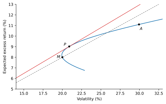
By (11), the active portfolio has an alpha of 3.88%, a beta of 0.90 and a residual volatility of 23.9%. By (12), w_{A}^{0} = (0.0388 / 0.0571) / (0.08 / 0.04) = 0.340 and w_{A}^{*} = 0.340 / (1 + (1 - 0.902) \times 0.340) = 0.329. The investor puts 32.9% of the portfolio in A and 67.1% in the market. The optimal portfolio has a beta of 0.97, an expected excess return of 9.02% and a volatility of 20.89%, for a Sharpe ratio of 0.432 against the market’s 0.400.

Figure 1 shows the geometry. The curve traces the portfolios that combine A and the market in different proportions. The active portfolio alone has a low Sharpe ratio, because most of its risk is residual, but mixed with the market its residual risk is diluted while its alpha still adds to the expected return. The optimal portfolio P is the point of the curve with the steepest capital allocation line, which lies above the market’s.

Figure 1: Expected excess return and volatility of portfolios that combine the active portfolio A of Example 1 with the market M. The optimal portfolio P has the steepest capital allocation line (solid). The dashed line is the capital allocation line of the market.

The Information Ratio

We can use (5) and (7) in (4) to get the expected return and the variance of the optimal portfolio: \operatorname{E}(R_{P}) = \lambda K, \qquad \sigma_{P}^{2} = \lambda^{2} K, \qquad K = \sum_{i = 1}^{N} \left(\frac{\alpha_{i}}{\sigma(e_{i})}\right)^{2} + \left(\frac{\operatorname{E}(R_{M})}{\sigma_{M}}\right)^{2}. \tag{13} The Sharpe ratio is therefore \sqrt{K}, which gives the following relationship between the Sharpe ratio of the optimal portfolio and the market Sharpe ratio, \left( \frac{\operatorname{E}(R_{P})}{\sigma_{P}} \right)^{2} = \sum_{i = 1}^{N} \left(\frac{\alpha_{i}}{\sigma(e_{i})}\right)^{2} + \left( \frac{\operatorname{E}(R_{M})}{\sigma_{M}} \right)^{2}. \tag{14} The equation shows that the Sharpe ratio of the optimal portfolio is higher than the Sharpe ratio of the market alone. Each security contributes positively, regardless of whether its alpha is positive or negative. Securities with negative alphas have negative weights, i.e., they are sold short in order to take advantage of the fact that they are expensive relative to the model.

For a given security i, the term \alpha_{i} / \sigma(e_{i}) is its information ratio, introduced in The Index Model, and it measures how good the alpha is. Treynor and Black call the alpha the appraisal premium and this ratio the appraisal ratio. If the volatility of the firm-specific risk is small, then it will be easier to diversify that risk away and hence extract the alpha of the security. Each security contributes to increasing the squared value of the Sharpe ratio of the optimal portfolio by the square of its information ratio. The active portfolio of (10) collects all of these contributions: its own squared information ratio, \alpha_{A}^{2} / \sigma^{2}(e_{A}), is the sum of the squared information ratios of its securities. In Example 1, the information ratios are 0.10, 0.10 and -0.08, and (14) gives a Sharpe ratio of \sqrt{0.10^{2} + 0.10^{2} + (-0.08)^{2} + 0.4^{2}} = 0.432, as before.

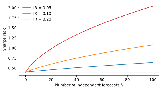
Since the contributions add up, many weak ideas can be worth as much as a few strong ones. With N independent forecasts that each have an information ratio of \mathit{IR}, the Sharpe ratio is \sqrt{S_{M}^{2} + N \, \mathit{IR}^{2}}, where S_{M} is the Sharpe ratio of the market. Figure 2 plots it. A single stock with an information ratio of 0.1 barely moves the Sharpe ratio of the market, but 25 of them raise it from 0.40 to 0.64. The information ratio of each forecast matters as much as their number: the same 25 forecasts with an information ratio of 0.05 raise the Sharpe ratio only to 0.47.

Figure 2: Sharpe ratio of the optimal portfolio with N independent forecasts that each have the same information ratio, when the market has a Sharpe ratio of 0.40.

Adjusting Alpha Forecasts

The model takes the alphas as known, but they are forecasts, and forecasts are noisy. Plugging a raw forecast into (5) treats it as if it were the true alpha. Suppose an analyst’s forecast is the true alpha plus an independent error, \alpha_{i}^{f} = \alpha_{i} + \varepsilon_{i}, and that across stocks the true alphas average zero. The best estimate of the true alpha given the forecast is then \hat{\alpha}_{i} = \frac{\sigma_{\alpha}^{2}}{\sigma_{\alpha}^{2} + \sigma_{\varepsilon}^{2}} \, \alpha_{i}^{f}, \tag{15} which shrinks the forecast toward zero, more so the noisier the forecasts are relative to the true dispersion of alphas. The shrinkage factor is the slope of a regression of true alphas on forecasts, and it can be estimated from the analyst’s record: regress the alphas that were realized on the forecasts that were made, and use the slope. Realized alphas are noisy too, but their noise is unrelated to the forecasts and does not bias the slope. Treynor and Black (1973) propose exactly this regression of realized returns, net of the market, on the analyst’s past estimates. Its intercept corrects an analyst who is persistently too optimistic or too pessimistic, and its slope one whose estimates are too extreme or too timid. This is the same logic as Estimation Risk and Shrinkage, applied to the alphas of the Treynor-Black model.

The adjustment matters more than it may seem. A forecast that is shrunk by a factor of 0.2 gets a fifth of the weight, and its contribution to the squared Sharpe ratio, the square of its information ratio, falls by a factor of 25. A raw forecast that is mostly noise does worse than nothing: as Problem 6 shows, it adds residual risk that no alpha compensates.

Historical Alphas as Forecasts

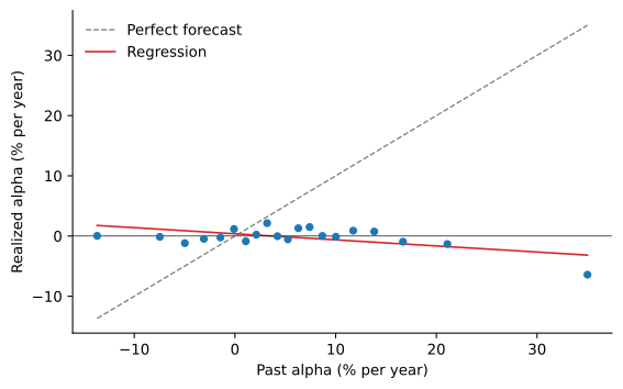
A tempting shortcut is to skip the analysts and use each stock’s alpha from an index-model regression on past returns, as in The Index Model. Each January from 1932 to 2025, we take the 100 largest U.S. stocks with returns in each of the previous 60 months and estimate their alphas, betas and residual variances over those months. The forecast is the past alpha. The realized alpha is the stock’s average return in excess of \beta_{i} R_{M} over the following year.

Figure 3 sorts the 9,385 stock-years into 20 groups by their forecast and plots the average realized alpha of each group. The average forecasts of the groups range from -14% to 35% a year, but the realized alphas show no relation to them, if anything a slightly negative one. The slope of the regression of realized on forecast alphas is -0.10, and the correlation -0.05. The slope is negative in 7 of the 10 decades. A large past alpha is mostly luck, and the stocks that did best over five years tend to do slightly worse afterwards.

Figure 3: Average realized alpha in the following year against the past 60-month alpha, for the 100 largest U.S. stocks each January from 1932 to 2025, in 20 groups sorted by past alpha. The dashed line is a perfect forecast and the solid line the regression of realized on past alphas across all stock-years. Annualized.

The consequence for the Treynor-Black portfolio is severe. From 1972 to 2025, we form the optimal portfolio each January from the raw forecasts, with the market’s expected excess return estimated by its average since 1926 and its variance over the previous 60 months, and hold it for the year. Past alphas look like excellent forecasts in the sample that produced them, with large information ratios, so the model takes enormous active positions. Table 2 summarizes the results. In the median year, the active positions add up to 7.5 times the portfolio’s value in absolute terms, financed in part by a short position in the market: the median weight in the market is -3.7. The portfolio’s volatility is 172% a year, and its Sharpe ratio, 0.25, is well below the market’s 0.48. In its worst month the portfolio lost 385% of its value, so an investor who followed it would have been wiped out. The statistics in the table treat each month’s return as if the investor could start over.

Table 2: Annualized excess returns of the market and of Treynor-Black portfolios of the 100 largest U.S. stocks formed each January from past 60-month alphas, 1972 to 2025.

	Mean (%)	Volatility (%)	Sharpe ratio	Worst month (%)
Market	7.57	15.77	0.48	-23.19
Raw forecasts	42.57	172.28	0.25	-385.19
Adjusted forecasts	7.57	15.77	0.48	-23.19

Adjusting the forecasts with (15) fixes the problem in the most direct way. Each January we estimate the slope of realized on forecast alphas from all earlier years. It is never positive, so the adjusted forecasts are zero, and the optimal portfolio is the market. That is the right answer. Past alphas carry no information about future alphas, and an investor who has no better forecasts should hold the market. The Treynor-Black model pays off only when the analysts’ forecasts have some accuracy, and the adjustment is what ensures that the portfolio bets only as much as that accuracy justifies.

Practice Problems

These problems give you a chance to practice the concepts introduced in this chapter. Try to solve each one on your own before expanding the solution.

Unless stated otherwise, the market has an expected excess return of \operatorname{E}(R_{M}) = 8\% and a volatility of \sigma_{M} = 20\%, so its Sharpe ratio is 0.40.

Problem 1 (Adding One Stock to the Market) Olivia Carter, a portfolio manager at Lakemont Investors, holds the market and believes Verdant Foods (VDF) has an alpha of 3\%, a beta of 1.2, and a residual volatility of 30\%.

1. Use (9) to compute \lambda, and find the weights in VDF and in the market.
2. Compute the beta, expected excess return, and volatility of the optimal portfolio, and its Sharpe ratio.
3. Check the Sharpe ratio with (14).

Solution

1. VDF has \alpha/\sigma^{2}(e) = 0.03/0.09 = 1/3, so \lambda = \frac{1}{0.08/0.04 + (1/3)(1 - 1.2)} = \frac{1}{1.9333} \approx 0.517. By (5) and (6), w_{VDF} = 0.517 \times 1/3 \approx 17.2\% and w_{M} \approx 82.8\%.

2. By (7), \beta_{P} = 0.517 \times 2 \approx 1.034, which matches 0.172 \times 1.2 + 0.828. By (4), \operatorname{E}(R_{P}) = 0.172 \times 0.03 + 1.034 \times 0.08 \approx 8.79\%, \qquad \sigma_{P} = \sqrt{1.034^{2} \times 0.04 + 0.172^{2} \times 0.09} \approx 21.3\%, so the Sharpe ratio is 0.0879/0.213 \approx 0.412.

3. VDF’s information ratio is 0.03/0.30 = 0.10, and (14) gives \sqrt{0.10^{2} + 0.40^{2}} = \sqrt{0.17} \approx 0.412. A 3\% alpha raises the Sharpe ratio only from 0.400 to 0.412, because it comes with 30\% of residual volatility.

Problem 2 (Profiting from a Negative Alpha) Olivia’s analysts now conclude that Brackley Retail (BRK) is overpriced: it has an alpha of -2\%, a beta of 0.9, and a residual volatility of 25\%. Consider a portfolio of BRK and the market only.

1. Find \lambda, the weight in BRK, and the weight in the market.
2. Does BRK raise or lower the Sharpe ratio of the portfolio? By how much?

Solution

1. BRK has \alpha/\sigma^{2}(e) = -0.02/0.0625 = -0.32, so \lambda = 1/(2 - 0.32 \times 0.1) = 1/1.968 \approx 0.508. Then w_{BRK} = 0.508 \times (-0.32) \approx -16.3\% and w_{M} \approx 116.3\%. Olivia sells BRK short and uses the proceeds to hold more than her wealth in the market.

2. It raises it. BRK’s information ratio is -0.02/0.25 = -0.08, and its square enters (14) with a positive sign: \sqrt{0.08^{2} + 0.40^{2}} \approx 0.408. An overpriced stock is as useful as an underpriced one, as long as it can be sold short.

Problem 3 (A Two-Stock Active Portfolio) Nathan Price at Westbury Capital combines the market with two stocks: Arlo Systems (ARS), with an alpha of 2\%, a beta of 1.2, and a residual volatility of 25\%; and Belmont Paper (BMP), with an alpha of -1\%, a beta of 0.8, and a residual volatility of 20\%.

1. Compute \lambda and the weights in ARS, BMP, and the market.
2. Compute the beta of the optimal portfolio in two ways, using (7) and using the weights.
3. Compute the Sharpe ratio of the optimal portfolio.

Solution

1. The ratios \alpha/\sigma^{2}(e) are 0.02/0.0625 = 0.32 for ARS and -0.01/0.04 = -0.25 for BMP, so \lambda = \frac{1}{2 + 0.32 \times (1 - 1.2) - 0.25 \times (1 - 0.8)} = \frac{1}{1.886} \approx 0.530. The weights are w_{ARS} = 0.530 \times 0.32 \approx 17.0\%, w_{BMP} = 0.530 \times (-0.25) \approx -13.3\%, and w_{M} = 1 - 0.170 + 0.133 \approx 96.3\%.

2. By (7), \beta_{P} = 0.530 \times 2 \approx 1.060. From the weights, 0.170 \times 1.2 - 0.133 \times 0.8 + 0.963 \approx 1.060.

3. The information ratios are 0.02/0.25 = 0.08 and -0.01/0.20 = -0.05, so by (14) the Sharpe ratio is \sqrt{0.0064 + 0.0025 + 0.16} \approx 0.411.

Problem 4 (Same Alpha, Different Risk) Two analysts at Westbury Capital each pitch a stock with an alpha of 2\%. Cresswell Labs (CRL) has a residual volatility of 10\%, and Duncan Exploration (DXP) has a residual volatility of 40\%.

1. How do the optimal weights of the two stocks compare?
2. By how much does each stock raise the squared Sharpe ratio of the optimal portfolio?

Solution

1. By (5), the weights are proportional to 0.02/0.01 = 2 for CRL and 0.02/0.16 = 0.125 for DXP, so CRL gets 16 times the weight of DXP. Four times the residual volatility means sixteen times the residual variance.

2. By (14), CRL adds (0.02/0.10)^{2} = 0.04 to the squared Sharpe ratio and DXP adds (0.02/0.40)^{2} = 0.0025. The two alphas are the same, but CRL’s is worth sixteen times as much.

Problem 5 (How Many Ideas Does a Fund Need?) Harriet Lowe is launching a fund that holds the market plus an active portfolio. Her research team can find stocks with information ratios of 0.05 in absolute value, independent of each other. How many such stocks does she need for the fund’s Sharpe ratio to reach 0.50?

Solution

By (14), N stocks raise the squared Sharpe ratio from 0.16 to 0.16 + N \times 0.05^{2}. Setting this equal to 0.50^{2} = 0.25 gives N = 0.09/0.0025 = 36. Each idea is weak on its own, and only a breadth of independent ideas adds up to a meaningful improvement.

Problem 6 (The Cost of False Alphas) Return to Nathan’s portfolio in Problem 3. Suppose his analysts were wrong, and the true alphas of ARS and BMP are both zero.

1. Using the same weights, what are the portfolio’s expected excess return and volatility?
2. Compare its Sharpe ratio with that of the market. What does the comparison say about acting on alpha forecasts?

Solution

1. Without alphas, the expected excess return is \beta_{P} \operatorname{E}(R_{M}) = 1.060 \times 0.08 \approx 8.48\%. The volatility does not depend on the alphas, so it is still about 21.8\%.

2. The Sharpe ratio is 0.0848/0.218 \approx 0.389, below the market’s 0.40. The active positions add firm-specific risk, and without true alphas nothing compensates for it. Alpha forecasts should be adjusted for how accurate they have been in the past before they are used to set positions.

Problem 7 (Monthly and Annual Information Ratios) A stock has an alpha of 0.25\% per month and a residual volatility of 5\% per month, with residuals independent from month to month. Compute its monthly and its annual information ratio.

Solution

The monthly information ratio is 0.0025/0.05 = 0.05. Over a year, the alpha adds up to 12 \times 0.25\% = 3\% while the residual volatility grows only to 5\% \times \sqrt{12} \approx 17.3\%, so the annual information ratio is 0.03/0.173 \approx 0.17 = 0.05 \times \sqrt{12}. Information ratios, like Sharpe ratios, grow with the square root of the horizon, so they should be compared over the same horizon.

Problem 8 (Choosing Between Two Managers) The Corliss Foundation holds the market and wants to add one market-neutral manager. Manager Xu promises an alpha of 4\% with a residual volatility of 20\%. Manager Yates promises an alpha of 2\% with a residual volatility of 5\%.

1. Compute each manager’s information ratio, and the Sharpe ratio the foundation could reach by combining the market with each manager optimally.
2. A trustee prefers Xu because his alpha is twice as large. How would you respond?

Solution

1. Xu’s information ratio is 0.04/0.20 = 0.2 and Yates’s is 0.02/0.05 = 0.4. By (14), the foundation reaches \sqrt{0.2^{2} + 0.4^{2}} \approx 0.447 with Xu and \sqrt{0.4^{2} + 0.4^{2}} \approx 0.566 with Yates.

2. The size of an alpha can be changed with leverage, but its quality cannot. Doubling the position with Yates gives an alpha of 4\% with a residual volatility of only 10\%, half of Xu’s risk for the same alpha. What matters is the alpha per unit of residual risk, and Yates offers twice as much.

Problem 9 (What Does a Sharpe Ratio Reveal?) A fund that holds the market plus an optimal active portfolio reports a Sharpe ratio of 0.55. What is the information ratio of its active portfolio, assuming the market’s Sharpe ratio is 0.40?

Solution

By (14), the squared information ratios of the active positions add up to 0.55^{2} - 0.40^{2} = 0.1425, so the active portfolio has an information ratio of \sqrt{0.1425} \approx 0.38.

Problem 10 (Two Steps for Two Stocks) Solve Problem 3 again in two steps.

1. Use (10) and (11) to find the weights of ARS and BMP in the active portfolio A, and its alpha, beta and residual variance.
2. Use (12) to find the weight of A in the optimal portfolio, and check the weights of ARS, BMP and the market against Problem 3.
3. Compute the information ratio of A and check it against the information ratios of the two stocks.

Solution

1. The ratios \alpha / \sigma^{2}(e) are 0.32 and -0.25, which add up to 0.07, so the weights in A are 0.32 / 0.07 = 4.571 for ARS and -0.25 / 0.07 = -3.571 for BMP. The active portfolio is a leveraged long-short position. Its alpha is 4.571 \times 0.02 + 3.571 \times 0.01 = 0.1271, its beta 4.571 \times 1.2 - 3.571 \times 0.8 = 2.629, and its residual variance 4.571^{2} \times 0.0625 + 3.571^{2} \times 0.04 = 1.816.

2. \alpha_{A} / \sigma^{2}(e_{A}) = 0.1271 / 1.816 = 0.07, so w_{A}^{0} = 0.07 / 2 = 0.035 and w_{A}^{*} = 0.035 / (1 - 1.629 \times 0.035) = 0.0371. The weights are 0.0371 \times 4.571 = 17.0\% in ARS, 0.0371 \times (-3.571) = -13.3\% in BMP and 1 - 0.0371 = 96.3\% in the market, as before. The high beta of A raises its weight from 3.5\% to 3.7\%.

3. 0.1271 / \sqrt{1.816} = 0.0943 = \sqrt{0.08^{2} + 0.05^{2}}. The squared information ratio of the active portfolio is the sum of those of its stocks.

Problem 11 (Adjusting a Forecast) An analyst forecasts an alpha of 4\% for a stock with a beta of 1 and a residual volatility of 20\%. A regression of the alphas realized on the analyst’s past forecasts has a slope of 0.25.

1. What is the adjusted alpha forecast?
2. Find the optimal weight in the stock with the raw and with the adjusted forecast.
3. Suppose the adjusted forecast is the true alpha. Compute the Sharpe ratio of each portfolio in (b) and compare them with the market’s.

Solution

1. By (15), 0.25 \times 4\% = 1\%.

2. With a beta of 1, (9) gives \lambda = 0.04 / 0.08 = 0.5, so the weight is 0.5 \times 0.04 / 0.04 = 50\% with the raw forecast and 0.5 \times 0.01 / 0.04 = 12.5\% with the adjusted one. The rest is in the market, and the portfolio’s beta is 1 either way.

3. With the raw weights, the expected excess return is 0.5 \times 0.01 + 0.08 = 8.5\% and the volatility \sqrt{0.04 + 0.5^{2} \times 0.04} = 22.4\%, a Sharpe ratio of 0.380. With the adjusted weights, they are 0.125 \times 0.01 + 0.08 = 8.125\% and \sqrt{0.04 + 0.125^{2} \times 0.04} = 20.2\%, a Sharpe ratio of 0.403 = \sqrt{0.40^{2} + 0.05^{2}}. The raw forecast bets four times too much and ends up below the market’s 0.40, while the adjusted forecast earns the best Sharpe ratio available.