Performance Evaluation

Why Measure Performance?

Investors hand money to managers because they hope the managers know something the market does not. Pension funds hire dozens of managers, individuals choose among thousands of mutual funds, and each year both decide whom to keep. Those decisions need a way to compare a fund’s record with what the investor could have earned without the manager. This chapter develops the tools: how to measure the return itself, how to adjust it for risk, how precise the answer is, and how to break the return into its sources. The Treynor-Black model already gives the logic of active management. Here we turn it around and ask how to tell, after the fact, whether a manager delivered.

Measuring the Return

Time-Weighted and Dollar-Weighted Returns

A fund’s return over many periods can be averaged in two ways. The time-weighted return compounds the return of each period, 1 + \bar{r}_{\text{TW}} = \left[ (1 + r_{1}) (1 + r_{2}) \cdots (1 + r_{T}) \right]^{1/T}, \tag{1} and is the return earned by $1 invested at the start and held to the end. It does not depend on how much money was in the fund at each date, so it measures what the manager did with each dollar.

The dollar-weighted return is the internal rate of return of the investor’s cash flows. If C_{0} is the initial investment, C_{t} the net amount the investor adds at the end of period t, and V_{T} the final value, the dollar-weighted return \bar{r}_{\text{DW}} solves C_{0} + \sum_{t = 1}^{T - 1} \frac{C_{t}}{(1 + \bar{r}_{\text{DW}})^{t}} = \frac{V_{T}}{(1 + \bar{r}_{\text{DW}})^{T}}. \tag{2} It gives more weight to the periods when more money was invested, so it measures what investors earned. The two differ when money flows in before bad returns or out before good ones. The manager controls the first and not the second, so performance evaluation uses time-weighted returns. The gap between the two is still worth knowing: it tells us how well investors timed their purchases of the fund.

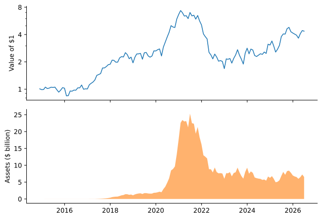
The ARK Innovation ETF is a vivid case. Figure 1 plots the growth of $1 invested at its launch, which is the time-weighted record, and the fund’s total assets. The fund compounded at 13.5% a year from November 2014 to June 2026. Its assets, though, were tiny during its best years and peaked at $25.3 billion in June 2021, after a spectacular 2020 and before the collapse of 2022. The dollar-weighted return of its investors as a group, computed from the monthly flows implied by its assets and returns, was -5.5% a year. In dollars, investors put in $10.6 billion more than they took out, and the fund’s assets at the end were $4.1 billion less than the money they had put in. The manager’s record and the investors’ experience tell different stories.

Figure 1: Growth of $1 invested in the ARK Innovation ETF at its launch, on a log scale (top), and the fund’s total net assets in billions of dollars (bottom).

Net and Gross Returns

Fund returns reported to investors are net of the fund’s expenses, which are deducted from its assets daily. Adding back the expense ratio gives the gross return, the return on the fund’s holdings. Gross returns measure whether the manager can pick stocks, net returns whether investors benefit. The data in this chapter come from the CRSP Survivor-Bias-Free U.S. Mutual Fund Database, whose returns are net of expenses but not of sales loads, and cover July 2006 to June 2026 unless stated otherwise.

Adjusting for Risk

A fund that earned 12% a year by holding twice the market’s risk has not done better than an index fund that earned 10%. Every risk-adjusted measure compares the fund with a passive alternative of the same risk, but they differ in which risk they hold fixed. Let R_{P} be the fund’s excess return over the risk-free rate, with mean \mu_{P}, volatility \sigma_{P}, market beta \beta_{P} and residual volatility \sigma(e_{P}) from the index model, and let the market have mean excess return \mu_{M} and volatility \sigma_{M}.

The Sharpe Ratio and M²

Sharpe (1966) proposed ranking funds by their reward-to-variability ratio, now the Sharpe ratio, \mathit{SR}_{P} = \frac{\mu_{P}}{\sigma_{P}}, \tag{3} the slope of the fund’s capital allocation line. An investor who can borrow and lend at the risk-free rate can reach any point on that line, so the fund with the steeper line offers the better tradeoff between mean and volatility.

Sharpe, William F. 1966. “Mutual Fund Performance.” Journal of Business 39 (1): 119–38.

Modigliani, Franco, and Leah Modigliani. 1997. “Risk-Adjusted Performance.” Journal of Portfolio Management 23 (2): 45–54.

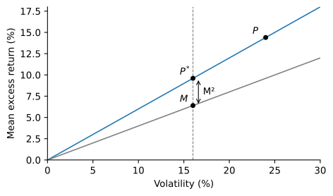
A ratio is hard to explain to a client. Modigliani and Modigliani (1997) turned it into a return: lever or unlever the fund with the risk-free asset until it has the market’s volatility, and compare its return with the market’s. A position of \sigma_{M}/\sigma_{P} in the fund has volatility \sigma_{M} and excess return \mu_{P} \sigma_{M} / \sigma_{P}, so the measure, usually called M², is M^{2}_{P} = \frac{\sigma_{M}}{\sigma_{P}} \mu_{P} - \mu_{M} = \sigma_{M} (\mathit{SR}_{P} - \mathit{SR}_{M}). \tag{4} It is expressed in percentage points of return and ranks funds exactly as the Sharpe ratio does. Figure 2 shows the construction: moving down the fund’s capital allocation line to the market’s volatility gives the portfolio P^{*}, and M² is the vertical distance between P^{*} and the market.

Figure 2: M² for a fund P with a higher Sharpe ratio than the market M. Combining the fund with T-bills moves along its capital allocation line to P^{*}, which has the market’s volatility, and M² is the difference between the mean excess returns of P^{*} and M.

Treynor’s Measure and Jensen’s Alpha

Treynor (1965) argued that a fund’s volatility is the wrong yardstick if the investor holds many funds. Firm-specific risk diversifies away across funds, and only market risk remains. Treynor’s measure divides the excess return by beta, T_{P} = \frac{\mu_{P}}{\beta_{P}}, \tag{5} the slope of the line from the risk-free asset to the fund in the plane of beta and expected return. The market’s value is T_{M} = \mu_{M}.

Treynor, Jack L. 1965. “How to Rate Management of Investment Funds.” Harvard Business Review 43 (1): 63–75.

Jensen, Michael C. 1968. “The Performance of Mutual Funds in the Period 1945–1964.” Journal of Finance 23 (2): 389–416.

Jensen (1968) measured performance instead by the intercept of the regression of the index model, R_{P,t} = \alpha_{P} + \beta_{P} R_{M,t} + e_{P,t}, \qquad \alpha_{P} = \mu_{P} - \beta_{P} \mu_{M}, \tag{6} which is the distance of the fund above the security market line. Jensen’s alpha is the return the fund earned beyond a passive portfolio of the market and T-bills with the same beta, and it comes with a t-statistic. The two measures are closely related: T_{P} - \mu_{M} = \alpha_{P} / \beta_{P}, so a fund beats the market on Treynor’s measure exactly when its alpha is positive. Applied to 115 mutual funds from 1945 to 1964, Jensen found that the funds on average could not predict prices well enough to outperform buying and holding the market, even when measured gross of management expenses, and that there was very little evidence that any individual fund did better than chance.

The Information Ratio

The information ratio scales the alpha by the residual risk that comes with it, \mathit{IR}_{P} = \frac{\alpha_{P}}{\sigma(e_{P})}. \tag{7} It is also known as the appraisal ratio. The Treynor-Black model shows why it matters: an investor who combines an active portfolio with the market, in the best proportions, raises the squared Sharpe ratio by the square of the active portfolio’s information ratio, \mathit{SR}^{2} = \mathit{SR}_{M}^{2} + \mathit{IR}_{P}^{2}. The alpha alone does not determine how much the fund is worth, because a large alpha with a lot of residual risk can be used only in small doses.

Which Measure?

Each measure answers a different question, and the right one depends on what else the investor holds.

The fund is	Use	Because
The investor’s whole risky portfolio	Sharpe ratio or M²	All of its volatility is borne
One of many funds held together	Treynor’s measure or alpha	Residual risk diversifies away
An active portfolio added to an index fund	Information ratio	It sets the gain in the overall Sharpe ratio

Example 1 (One Fund, Three Verdicts) The market has an expected excess return of 7\% and a volatility of 18\%, so \mathit{SR}_{M} = 0.389. A fund has an excess return of 9\%, a volatility of 25\% and a beta of 1.2. Its measures are \begin{aligned} \mathit{SR}_{P} & = \frac{9\%}{25\%} = 0.36, &\qquad M^{2}_{P} & = 18\% \times (0.36 - 0.389) = -0.52\%, \\ T_{P} & = \frac{9\%}{1.2} = 7.5\%, &\qquad \alpha_{P} & = 9\% - 1.2 \times 7\% = 0.6\%. \end{aligned} Its residual variance is 0.25^{2} - 1.2^{2} \times 0.18^{2} = 0.0158, so \sigma(e_{P}) = 12.6\% and \mathit{IR}_{P} = 0.6 / 12.6 = 0.048. As the only risky holding, the fund is worse than the market: its Sharpe ratio is lower. As one of many funds, it is better: its Treynor measure exceeds 7\% and its alpha is positive. As an addition to an index fund, it is nearly worthless: its information ratio raises the squared Sharpe ratio from 0.151 to 0.153.

Measures for Real Funds

Table 1 reports the measures for eight well-known funds over the last twenty years: the Vanguard 500 Index Fund, three growth funds (Fidelity Magellan, Fidelity Contrafund and T. Rowe Price Growth Stock), two value funds (Vanguard Windsor and Dodge & Cox Stock), and two funds that follow neither label (Vanguard Primecap and Sequoia). All numbers are annualized. The market is the value-weighted portfolio of U.S. stocks.

Table 1: Annualized performance measures from net returns, July 2006 to June 2026. Mean is the average excess return over T-bills; mean, volatility, M², Treynor’s measure and alpha are in percent; t is the t-statistic of alpha and IR the information ratio.

	Mean	Vol.	Sharpe	M²	Beta	Treynor	Alpha	t	IR
Vanguard 500	10.3	15.3	0.67	0.1	0.97	10.7	0.1	0.39	0.09
Magellan	9.5	17.9	0.53	-2.2	1.08	8.8	-1.9	-1.52	-0.35
Contrafund	12.0	15.5	0.77	1.6	0.93	12.9	2.2	1.87	0.43
Growth Stock	11.2	17.7	0.63	-0.6	1.05	10.7	0.2	0.11	0.03
Windsor	8.4	17.1	0.49	-2.8	1.02	8.2	-2.3	-1.76	-0.40
Dodge & Cox	8.7	17.6	0.49	-2.8	1.04	8.3	-2.3	-1.56	-0.36
Primecap	12.5	15.9	0.78	1.8	0.96	13.0	2.4	2.10	0.48
Sequoia	7.5	16.3	0.46	-3.2	0.85	8.8	-1.4	-0.68	-0.16
Market	10.5	15.8	0.67	0.0	1.00	10.5

The rankings mostly agree. Vanguard Primecap and Fidelity Contrafund top every measure, with Sharpe ratios of 0.78 and 0.77 against 0.67 for the market, and the two value funds and Magellan sit at the bottom. The agreement is not a coincidence. These are diversified stock funds with betas near one and R-squared values around 0.9, so volatility and beta convey nearly the same information. The exception is Sequoia, a concentrated fund with a beta of 0.85. Its Treynor measure ranks it with Magellan, while its Sharpe ratio ranks it last, because it carries much more residual risk. Which ranking matters depends on whether Sequoia is an investor’s only fund.

The index fund deserves a look. Its alpha of 0.13% a year is indistinguishable from zero, but its beta is 0.97 and its R-squared is below one. The S&P 500 holds large firms only, while the benchmark here is the whole market, so even a perfect index fund does not track it exactly.

Multifactor Alphas

A fund whose CAPM alpha comes from tilting toward small stocks, value stocks or past winners has not shown skill, because an investor could buy those tilts cheaply through index funds or factor portfolios. Following Carhart (1997), studies of fund performance measure alpha against factor models. Table 2 reports the loadings of each fund on the six factors of Fama and French (2018).

Carhart, Mark M. 1997. “On Persistence in Mutual Fund Performance.” Journal of Finance 52 (1): 57–82.

Fama, Eugene F., and Kenneth R. French. 2018. “Choosing Factors.” Journal of Financial Economics 128 (2): 234–52.

Table 2: Six-factor regressions of the funds’ monthly excess returns, July 2006 to June 2026. Alphas are annualized, in percent.

	Alpha	t	MKT	SMB	HML	RMW	CMA	UMD	R^{2}
Vanguard 500	-0.33	-1.83	1.00	-0.12	0.03	0.05	0.02	-0.00	1.00
Magellan	-2.28	-2.07	1.11	-0.09	-0.14	-0.02	-0.14	0.02	0.93
Contrafund	1.08	1.25	0.98	-0.09	-0.15	0.07	-0.18	0.09	0.94
Growth Stock	-0.17	-0.18	1.07	-0.06	-0.29	-0.06	-0.27	0.01	0.95
Windsor	-1.24	-1.37	0.96	0.09	0.26	0.01	0.11	-0.09	0.95
Dodge & Cox	-1.29	-1.28	0.98	0.01	0.31	0.04	0.09	-0.11	0.94
Primecap	2.57	2.28	0.97	-0.05	0.05	-0.13	-0.03	0.04	0.91
Sequoia	-1.14	-0.53	0.81	0.14	0.05	0.12	-0.15	-0.02	0.69

The loadings describe each fund’s style without looking at its holdings. The growth funds load negatively on HML and CMA: they hold expensive firms that invest heavily. Windsor and Dodge & Cox load positively on HML. Their CAPM alphas, around -2.3% a year, partly reflect the poor returns of value stocks since 2007, and against the six factors they shrink to about -1.2%. Magellan’s alpha, on the other hand, gets worse, to -2.3% a year with a t-statistic of -2.07. Primecap is the only fund with a significant positive alpha under both models. The index fund’s SMB loading of -0.12 captures the large-firm tilt that pushed its beta below one, and its six-factor alpha of -0.33% is small and negative, as an index fund’s should be after its 0.15% expense ratio and trading costs.

How Precise Is a Measured Alpha?

The estimated alpha of (6) has a standard error of about \sigma(e_{P})/\sqrt{T} when measured over T years, so its t-statistic is approximately t(\hat{\alpha}_{P}) \approx \frac{\alpha_{P}}{\sigma(e_{P}) / \sqrt{T}} = \mathit{IR}_{P} \sqrt{T}. \tag{8} To reach a t-statistic of 2, a manager needs T = (2 / \mathit{IR}_{P})^{2} years of returns. A manager with an information ratio of 0.5, which would be excellent, needs 16 years; one with 0.25 needs 64. Primecap’s information ratio of 0.48 over 20 years gives 2.15 by (8), close to the regression’s 2.10. Twenty years is long for a manager’s career, and enough to establish only the very best records.

Sharpe ratios are no more precise. Lo (2002) shows that if returns are independent and identically distributed, the estimated Sharpe ratio from T periods has an approximate standard error of \operatorname{SE}(\widehat{\mathit{SR}}) = \sqrt{\frac{1 + \mathit{SR}^{2} / 2}{T}}, \tag{9} in the units of the period. The market’s monthly Sharpe ratio over our 240 months was 0.193, so its standard error is 0.065 a month, or 0.23 annualized. A 95% confidence interval for the market’s annual Sharpe ratio runs from 0.23 to 1.11, and every fund in Table 1 falls inside it. Lo also shows that annualizing by \sqrt{12} is valid only if returns are serially uncorrelated. Returns of hedge funds, whose illiquid holdings are marked to stale prices, are positively autocorrelated, and Lo finds that their annual Sharpe ratios can be overstated by as much as 65%.

Lo, Andrew W. 2002. “The Statistics of Sharpe Ratios.” Financial Analysts Journal 58 (4): 36–52.

Style Analysis

Sharpe (1992) proposed a way to find a fund’s benchmark from its returns alone. Choose n asset classes, each represented by an index that can be held cheaply, and find the mix of them that tracks the fund most closely: r_{P,t} = \sum_{j = 1}^{n} w_{j} r_{j,t} + e_{P,t}, \qquad \min_{w} \operatorname{V}(e_{P}) \quad \text{subject to} \quad \sum_{j = 1}^{n} w_{j} = 1, \quad w_{j} \geq 0. \tag{10} The constraints make the mix a portfolio an investor could hold without leverage or short sales, its style. The return of the mix is the return attributable to style, and the residual e_{P,t} is the return due to selection. Sharpe used twelve asset classes covering bonds, stocks and cash. For U.S. stock funds, the four Vanguard index funds of large and small, value and growth stocks, together with T-bills, are a natural set: each of them is a low-cost fund an investor could have bought instead.

Sharpe, William F. 1992. “Asset Allocation: Management Style and Performance Measurement.” Journal of Portfolio Management 18 (2): 7–19.

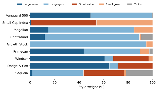
Figure 3 shows the style weights of the eight funds and of the Vanguard Small-Cap Index Fund. The two index funds are a check on the method. The S&P 500 fund comes out as 49% large value and 50% large growth, with an R-squared of 0.998, and the small-cap index fund as 54% small value and 46% small growth. Both are what their holdings say they should be. T. Rowe Price Growth Stock is almost pure large growth, Windsor and Dodge & Cox are about two-thirds large value and one-third small value, and Sequoia’s style includes 22% T-bills, with an R-squared of only 0.69.

Figure 3: Style weights of seven active funds and two index funds, estimated with (10) on monthly returns of four Vanguard index funds and T-bills.

The selection return is the fund’s return minus the return of its style mix. Since both the fund and the index funds report net returns, it measures what the active fund added after costs relative to a passive alternative with the same style. Primecap’s selection return was 2.4% a year with a t-statistic of 2.19, and Contrafund’s 1.3% (t = 1.53). Magellan’s was -1.9% (t = -1.84). The weights are estimated with the same returns they are used to evaluate, so the style mix is chosen with hindsight. Sharpe recommended measuring selection out of sample instead, comparing each month’s return with a style mix estimated from earlier returns only.

Changing Risk and Market Timing

Every measure so far assumes the fund’s risk is constant. A manager who forecasts the market will not keep it constant, but will raise the fund’s beta before markets expected to rise and lower it before markets expected to fall. If the forecasts are good, the fund’s return is a convex function of the market’s, and a straight-line regression misreads it.

Treynor and Mazuy (1966) proposed testing for this curvature by adding a squared term to the regression, R_{P,t} = \alpha_{P} + \beta_{P} R_{M,t} + \gamma_{P} R_{M,t}^{2} + e_{P,t}, \tag{11} where a positive \gamma_{P} indicates successful timing. In 57 funds they found no evidence that fund managers could outguess the market.

Treynor, Jack L., and Kay K. Mazuy. 1966. “Can Mutual Funds Outguess the Market?” Harvard Business Review 44: 131–36.

Henriksson, Roy D., and Robert C. Merton. 1981. “On Market Timing and Investment Performance. II. Statistical Procedures for Evaluating Forecasting Skills.” Journal of Business 54 (4): 513–33.

Henriksson and Merton (1981) modeled a timer who forecasts only whether the market will beat T-bills, and holds a beta of \beta_{\text{up}} after an up forecast and \beta_{\text{down}} after a down forecast. With perfect forecasts, the fund’s excess return is \beta_{\text{up}} R_{M} when R_{M} > 0 and \beta_{\text{down}} R_{M} when R_{M} \leq 0, which can be written as \beta_{\text{up}} R_{M} + (\beta_{\text{up}} - \beta_{\text{down}}) \max(-R_{M}, 0). With imperfect forecasts this suggests the regression R_{P,t} = \alpha_{P} + \beta_{P} R_{M,t} + c_{P} \max(-R_{M,t}, 0) + e_{P,t}. \tag{12} The term \max(-R_{M}, 0) is the payoff of a put option on the market with a strike equal to the risk-free return. A positive c_{P} means the timer has given investors c_{P} such puts for free, and c_{P} times the market price of the put is an estimate of the value of the timing ability.

Over our sample, seven of the eight funds have a negative \gamma_{P} in (11), and none of the positive estimates is significant. This matches a long line of studies, summarized by Ferson and Schadt (1996), in which the typical fund looks like a perverse timer, with more market exposure before low market returns. Ferson and Schadt argue that much of this reflects public information rather than bad forecasts. Dividend yields and interest rates predict market returns, and a fund’s beta can move with the same variables for reasons unrelated to skill. They suggest one mechanism: new money flows into funds when the public expects high returns, managers take time to invest it, and the extra cash lowers the fund’s beta at those times. Their conditional measures let beta depend on lagged public information, and with them the distribution of fund alphas is consistent with neutral performance and the evidence of perverse timing goes away.

Ferson, Wayne E., and Rudi W. Schadt. 1996. “Measuring Fund Strategy and Performance in Changing Economic Conditions.” Journal of Finance 51 (2): 425–61.

Convexity can also come from holdings rather than forecasts. A fund that buys options, or stocks whose payoffs behave like options, will show a positive \gamma_{P} without any ability to time the market, and a fund that sells options will show a negative one. Alpha and the timing coefficient have to be read together: a fund that buys puts pays for the convexity, which shows up as a lower alpha.

Performance Attribution

A pension plan or a balanced fund invests across asset classes. Its sponsor sets a policy, the long-run weight of each class, and the managers deviate from it in two ways: by changing the weights from period to period, timing in the sense of Brinson et al. (1986), and by choosing securities within each class, selection. Let w_{P,j} and w_{B,j} be the actual and policy weights of class j, and r_{P,j} and r_{B,j} the fund’s return in that class and the return of the class’s index. Four portfolio returns separate the effects:

Brinson, Gary P., L. Randolph Hood, and Gilbert L. Beebower. 1986. “Determinants of Portfolio Performance.” Financial Analysts Journal 42 (4): 39–44.

	Index returns	Actual returns
Policy weights	I: \sum_{j} w_{B,j} r_{B,j}	III: \sum_{j} w_{B,j} r_{P,j}
Actual weights	II: \sum_{j} w_{P,j} r_{B,j}	IV: \sum_{j} w_{P,j} r_{P,j}

Portfolio I is the policy return, II adds timing to the policy, III adds selection, and IV is the fund’s actual return. The contribution of timing is II - I, that of selection is III - I, and the remainder IV - III - II + I is an interaction term. The three add up to the difference between the actual return and the policy return.

Example 2 (Attributing a Balanced Fund’s Return) A fund’s policy is 60% stocks, 30% bonds and 10% cash. Over the year the stock index returned 8%, the bond index 3% and cash 1%. The fund held 70% stocks, 25% bonds and 5% cash, and its stocks returned 9%, its bonds 2.5% and its cash 1%. In percent, the four portfolios return \begin{aligned} \text{I} & = 0.6 (8) + 0.3 (3) + 0.1 (1) = 5.8\%, &\qquad \text{II} & = 0.7 (8) + 0.25 (3) + 0.05 (1) = 6.4\%, \\ \text{III} & = 0.6 (9) + 0.3 (2.5) + 0.1 (1) = 6.25\%, &\qquad \text{IV} & = 0.7 (9) + 0.25 (2.5) + 0.05 (1) = 6.975\%. \end{aligned} The fund beat its policy by 1.175\%: timing contributed 0.6\%, by overweighting stocks in a year when they beat bonds and cash, selection 0.45\%, and the interaction 0.125\%, the extra gain from overweighting stocks in the class where selection was good.

Brinson, Hood and Beebower applied this framework to 91 large U.S. pension plans from 1974 to 1983. The plans’ average annual return was 9.01%, against 10.11% for their policy portfolios, so active management cost them about 1.1% a year. And investment policy explained on average 93.6% of the variation of each plan’s quarterly returns over time. The second number is often quoted as saying that asset allocation explains 94% of the differences in returns across funds, which is not what they measured. A plan’s returns move with markets mainly because of its policy weights, but two plans with similar policies can still earn quite different returns.

Benchmarks from Holdings

Factor regressions and style analysis infer a fund’s exposures from its returns. When the holdings are known, the benchmark can be built from them instead. Daniel et al. (1997) match each stock a fund holds with one of 125 passive portfolios formed on size, book-to-market and prior-year return, the characteristics of the anomalies, and decompose the fund’s return into three parts. Characteristic selectivity (CS) is the return of each stock minus the return of its matching portfolio, weighted by the fund’s holdings. Characteristic timing (CT) measures whether the fund shifted toward characteristics just before they paid off. Average style (AS) is the return the fund would have earned by holding its average characteristics. In over 2,500 equity funds from 1975 to 1994, they find some selectivity ability, particularly among aggressive-growth funds, and no characteristic timing ability. What the funds added through CS and CT is statistically significant but not larger than the difference between active and passive fund expenses.

Daniel, Kent, Mark Grinblatt, Sheridan Titman, and Russ Wermers. 1997. “Measuring Mutual Fund Performance with Characteristic-Based Benchmarks.” Journal of Finance 52 (3): 1035–58.

Gaming the Measures

A measure that managers are paid on is a measure they will try to raise. Goetzmann et al. (2007) show that the Sharpe ratio, Jensen’s alpha and the timing measures can all be raised by trading strategies that use no information about the assets. Changing leverage after a run of good or bad returns, or buying and selling options, changes the distribution of returns in ways that these measures, designed for normally distributed returns, misread. In their simulations, simple strategies that relever the portfolio each period or trade liquid at-the-money options produce seemingly spectacular results, even with very high transaction costs. The risk is greatest for hedge funds, which are free to use options and leverage.

Goetzmann, William, Jonathan Ingersoll, Matthew Spiegel, and Ivo Welch. 2007. “Portfolio Performance Manipulation and Manipulation-Proof Performance Measures.” Review of Financial Studies 20 (5): 1503–46.

They show that, under some conditions, a measure that cannot be manipulated this way must take the form \hat{\Theta} = \frac{1}{(1 - \rho) \Delta t} \ln \left[ \frac{1}{T} \sum_{t = 1}^{T} \left( \frac{1 + r_{t}}{1 + r_{f,t}} \right)^{1 - \rho} \right], \tag{13} where r_{t} is the fund’s return in period t, \Delta t the length of a period in years, and \rho a coefficient of risk aversion. The bracket is the average power utility of the fund’s returns relative to T-bills, and \hat{\Theta} is the annualized continuously compounded excess return of a risk-free asset that gives the same utility, a certainty equivalent. They recommend choosing \rho so that, absent information, holding the market is the best a manager can do, and use \rho = 3 in their simulations. Their example: a fund with monthly returns of -10\%, 5\%, 17\% and -2\% when T-bills pay 1% a month has \hat{\Theta} = 6.6\% with \rho = 2 and 1.2\% with \rho = 3. The measure is nearly the same as the Morningstar Risk-Adjusted Return used in Morningstar’s star ratings, which sets \rho = 3.

Table 3 computes \hat{\Theta} for the funds of Table 1. In the limit \rho \to 1 the measure becomes the average log return relative to T-bills, so \hat{\Theta} is the fund’s continuously compounded return over T-bills. Raising \rho to 3 charges for volatility. For returns close to lognormal the charge is about (\rho - 1) \sigma^{2} / 2, which costs the funds between 2.4 and 3.4 percentage points a year, the most for Magellan, the most volatile of them.

Table 3: Sharpe ratio and the manipulation-proof measure (13) of the funds, from monthly net returns, July 2006 to June 2026. \hat{\Theta} is in percent per year.

	Sharpe	\hat{\Theta}, \rho = 1	\hat{\Theta}, \rho = 3
Vanguard 500	0.67	9.09	6.67
Magellan	0.53	7.85	4.47
Contrafund	0.77	10.69	8.24
Growth Stock	0.63	9.57	6.33
Windsor	0.49	6.90	3.89
Dodge & Cox	0.49	7.08	3.84
Primecap	0.78	11.16	8.56
Sequoia	0.46	6.16	3.35
Market	0.67	9.23	6.68

The ranking by \hat{\Theta} with \rho = 3 is nearly the same as the ranking by Sharpe ratio. Primecap and Contrafund are still first and second, and Sequoia is still last. The only funds that trade places are Windsor and Dodge & Cox, whose \hat{\Theta} differ by 0.05 points. That is what we should expect. These are diversified stock funds that do not trade options or change their leverage much, so their returns are close to normal, and for such returns the Sharpe ratio and \hat{\Theta} measure nearly the same thing. The measure earns its keep on strategies whose returns are far from normal, which a table of mutual funds does not contain. In our sample, the rule of choosing \rho so that levering the market up or down does not raise \hat{\Theta} gives \rho = 4.0, close to the value of 3 that Goetzmann et al. and Morningstar use.

Practice Problems

These problems give you a chance to practice the concepts introduced in this chapter. Try to solve each one on your own before expanding the solution.

Problem 1 (Time-Weighted and Dollar-Weighted Returns) The Larkspur Growth Fund starts the year with $100 million. It returns 50\% in its first year, and after its strong record investors add $150 million at the end of that year. In the second year it returns -20\%.

1. Compute the fund’s time-weighted return per year.
2. Compute the dollar-weighted return of the fund’s investors.
3. How much money did investors gain or lose in total? Which return describes the manager, and which the investors?

Solution

1. By (1), 1 + \bar{r}_{\text{TW}} = (1.5 \times 0.8)^{1/2} = 1.0954, so \bar{r}_{\text{TW}} = 9.54\% a year.

2. The fund has $150 million at the end of the first year and $300 million after the inflow, so it ends with 0.8 \times 300 = \$240 million. By (2), with x = 1 + \bar{r}_{\text{DW}}, 100 + \frac{150}{x} = \frac{240}{x^{2}} \quad \Longrightarrow \quad 100 x^{2} + 150 x - 240 = 0 \quad \Longrightarrow \quad x = \frac{-150 + \sqrt{150^{2} + 4 \times 100 \times 240}}{200} = 0.9712, so \bar{r}_{\text{DW}} = -2.88\% a year.

3. Investors put in $250 million and ended with $240 million, a loss of $10 million. The time-weighted return describes the manager, who earned 9.54\% a year on each dollar in the fund. The dollar-weighted return describes the investors, who put most of their money in just before the bad year.

Problem 2 (Choosing a Fund) The market has an expected excess return of 8\% and a volatility of 20\%. Three funds have the following characteristics:

Fund	Excess return	Volatility	Beta
Alder	10%	26%	1.2
Birch	7%	15%	0.7
Cedar	9.5%	30%	0.9

1. Compute the Sharpe ratio, Treynor’s measure, Jensen’s alpha and the information ratio of each fund.
2. Which fund should an investor choose if it will be the only risky investment?
3. Which fund should a pension plan choose if it will be one of many managers it hires?
4. Which fund is the best complement to an index fund?

Solution

1. The market’s Sharpe ratio is 0.40. Residual volatilities follow from \sigma^{2}(e) = \sigma^{2} - \beta^{2} \sigma_{M}^{2}.

   Fund	Sharpe	Treynor	Alpha	\sigma(e)	IR
   Alder	0.385	8.33%	0.4%	10.0%	0.040
   Birch	0.467	10.0%	1.4%	5.39%	0.260
   Cedar	0.317	10.56%	2.3%	24.0%	0.096

   For example, Cedar’s alpha is 9.5\% - 0.9 \times 8\% = 2.3\% and \sigma^{2}(e) = 0.09 - 0.81 \times 0.04 = 0.0576.

2. As the only risky investment, the fund’s total volatility matters, so the investor should pick the highest Sharpe ratio, Birch. Its M² is 20\% \times (0.467 - 0.40) = 1.33\%. Alder and Cedar have Sharpe ratios below the market’s.

3. Across many managers, residual risk diversifies away, and Treynor’s measure and alpha are the relevant measures. Cedar has the highest of both.

4. Combined with an index fund, the information ratio determines the gain in the Sharpe ratio, so Birch is the best complement. With it, the squared Sharpe ratio rises from 0.16 to 0.16 + 0.26^{2} = 0.228, a Sharpe ratio of 0.477. Cedar’s large alpha comes with too much residual risk to be used in a large position.

Problem 3 (How Long Does It Take?) Maren Holt runs a stock fund with an alpha of 1.5\% a year and a residual volatility of 5\%.

1. What is Maren’s information ratio? How many years of returns are needed for the alpha to have a t-statistic of 2?
2. A rival manager has an alpha of 3\% with a residual volatility of 12\%. How many years does the rival need?
3. A consultant evaluates managers on five-year records. What t-statistic should the consultant expect for Maren’s alpha after five years?

Solution

1. \mathit{IR} = 1.5\% / 5\% = 0.3. By (8), T = (2/0.3)^{2} = 44 years.

2. \mathit{IR} = 3\% / 12\% = 0.25, so T = (2/0.25)^{2} = 64 years. His alpha is twice as large, but it comes with more than twice the residual risk.

3. t \approx 0.3 \times \sqrt{5} = 0.67. A five-year record cannot separate a manager with a real information ratio of 0.3 from one with none.

Problem 4 (Attribution of a Pension Plan) A pension plan’s policy is 50% stocks, 40% bonds and 10% cash. In one year the stock index returned 10%, the bond index 4% and cash 2%. The plan held 40% stocks, 50% bonds and 10% cash, and its stock managers returned 11%, its bond managers 4.5%, and its cash 2%.

1. Compute the plan’s return and the return of its policy.
2. Decompose the difference into timing, selection and interaction.
3. What should the plan’s investment committee conclude?

Solution

1. The actual return is 0.4 \times 11\% + 0.5 \times 4.5\% + 0.1 \times 2\% = 6.85\% and the policy return 0.5 \times 10\% + 0.4 \times 4\% + 0.1 \times 2\% = 6.8\%.

2. Portfolio II is 0.4 \times 10\% + 0.5 \times 4\% + 0.1 \times 2\% = 6.2\% and portfolio III is 0.5 \times 11\% + 0.4 \times 4.5\% + 0.1 \times 2\% = 7.5\%. Timing contributed 6.2\% - 6.8\% = -0.6\%, selection 7.5\% - 6.8\% = 0.7\%, and the interaction 6.85\% - 6.2\% - 7.5\% + 6.8\% = -0.05\%. The three add up to 0.05\%.

3. The plan barely beat its policy, but for two offsetting reasons. Underweighting stocks in a year when they beat bonds cost 0.6\%, while the security selection of its managers added 0.7\%. One year is far too short to judge either, but the committee should ask who decided to underweight stocks and on what basis.

Problem 5 (A Market Timer) Teodor Vance runs a fund that holds a beta of 1.3 after forecasting that the market will beat T-bills and 0.7 otherwise, and the forecasts are always right.

1. Write the fund’s excess return as a function of the market’s excess return in the form of (12). What are \beta_{P} and c_{P}?
2. A one-year put on the market with a strike equal to the risk-free return costs 6\% of the market’s value. What is Teodor’s timing ability worth per year?
3. What sign would you expect for \gamma_{P} in the Treynor-Mazuy regression (11) of the fund’s returns? What would the regression report if the forecasts were right only half the time?

Solution

1. When R_{M} > 0, R_{P} = 1.3 R_{M}; when R_{M} \leq 0, R_{P} = 0.7 R_{M}. Both are captured by R_{P} = 1.3 R_{M} + 0.6 \max(-R_{M}, 0), since in down markets 1.3 R_{M} - 0.6 R_{M} = 0.7 R_{M}. So \beta_{P} = 1.3 and c_{P} = 1.3 - 0.7 = 0.6.

2. The fund gives investors 0.6 puts for free each year, worth 0.6 \times 6\% = 3.6\% of the fund’s value.

3. The fund’s return is a convex function of the market’s, so \gamma_{P} > 0. If the forecasts were right only half the time, the beta would be unrelated to the market’s return: the regression would find c_{P} and \gamma_{P} close to zero and a beta near the average of 1.0.

Problem 6 (Selection after Style) A style analysis of the Hawthorne Equity Fund over the past five years gives weights of 70\% on a large growth index fund and 30\% on a small value index fund, with an R-squared of 0.95. This year the large growth index fund returned 14\%, the small value index fund 6\%, and the Hawthorne fund 12\%. All returns are net of expenses.

1. Compute the fund’s style return and its selection return for the year.
2. The fund advertises that it beat the S&P 500, which returned 10\%. Is that the right comparison?
3. Why does style analysis require the weights to be nonnegative and sum to one?

Solution

1. The style return is 0.7 \times 14\% + 0.3 \times 6\% = 11.6\%, so the selection return is 12\% - 11.6\% = 0.4\%.

2. No. The fund’s style is mostly large growth, which beat the S&P 500 this year. An investor could have earned 11.6\% with two index funds, so the manager added only 0.4\%, and one year of selection returns says little about skill.

3. The constraints make the style mix a portfolio that an investor can hold without borrowing or short selling, so the style return is a real alternative. An unconstrained regression could fit the fund better with weights that no investor would hold, and its residual would no longer measure what the manager added over a feasible passive strategy.