| Monthly Estimate (%) | Annualized Estimate (%) | |
|---|---|---|
| Mean | 2.25 | 27.05 |
| St. Dev. | 12.47 | 43.19 |
Statistics of Asset Returns
Investment performance begins with a simple question: what payoff does each dollar invested generate? The holding-period return (HPR) answers this question. Because future prices and cash flows are uncertain, returns are random variables whose most important characteristics are their expected return and volatility. Applying the law of one price to portfolios shows that portfolio returns are simply weighted averages of asset returns, and ETF arbitrage shows how this theoretical principle underpins an entire industry.
Financial and Real Assets
Investing exchanges wealth today for future payoffs. Even if you plan to hold an asset indefinitely, marking its price at the end of each period lets you evaluate performance one period at a time.
An asset can be real, like a house, or financial, like a stock or bond. Financial assets are claims on real assets or the income they generate. Because one party’s financial asset is another party’s liability, financial claims net to zero across the economy; real assets constitute society’s net wealth.
Assets may also distribute cash while you hold them. Stocks pay dividends, bonds pay coupons, and rental properties generate rent.
The Rate of Return
Suppose you buy an asset at time 0 for P_{0}, receive a cash distribution D_{1} during the period, and value or sell the asset at time 1 for P_{1}. Its ending payoff is P_{1}+D_{1}, and its holding-period return (HPR) is \text{HPR} = \frac{P_{1} - P_{0} + D_{1}}{P_{0}}. Equivalently, \text{HPR} = \frac{P_{1} - P_{0}}{P_{0}} + \frac{D_{1}}{P_{0}}. The first term is the capital-gain yield and the second is the income yield. Together they measure the asset’s total return. For stocks, whose cash distribution is a dividend, the income yield is called the dividend yield.
Example 1 Suppose you purchase today an index fund for $100 per share. The fund will pay dividends over a year of $4. If the price per share next year is $110, your HPR amounts to \text{HPR} = \frac{110 - 100 + 4}{100} = 14\%. The 14% total return consists of a 10% capital-gain yield and a 4% dividend yield.
Let r_{i} denote the HPR of asset i. Because its future price and distributions are uncertain, r_{i} is a random variable on a probability space (\Omega, \operatorname{P}). Probability Basics in Stochastic Foundations for Finance reviews random variables and their statistical moments.
The expectation of r_i is its expected return, and its standard deviation is its volatility. We write \begin{aligned} \mu_{i} & = \operatorname{E}(r_{i}), \\ \sigma_{i} & = \sqrt{\operatorname{V}(r_{i})}. \end{aligned}
Example 2 Suppose your expectations regarding a stock price are as follows:
| State of the Market | Probability | HPR |
|---|---|---|
| Boom | 0.35 | 44.5% |
| Normal | 0.30 | 14% |
| Recession | 0.35 | -16.5% |
We can compute the mean and standard deviation of the stock’s HPR as \begin{aligned} \mu & = 0.35 \times 0.445 + 0.3 \times 0.14 + 0.35 \times (-0.165) = 14\%, \\ \sigma & = \sqrt{0.35 \times (0.445 - 0.14)^{2} + 0.3 \times (0.14 - 0.14)^{2} + 0.35 \times (-0.165 - 0.14)^{2}} \\ & = 25.52\%. \end{aligned}
Stock Returns
The previous example assumed known state probabilities. In practice, we usually estimate return moments from historical data.
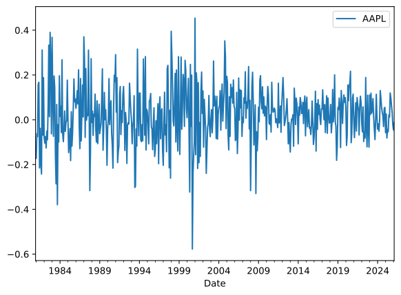
Figure 1 shows Apple’s monthly returns since its December 1980 listing. Returns fluctuate substantially, and their volatility changes over time. The sample mean is1 \bar{r} = \frac{1}{N} \sum_{t = 1}^{N} r_{t}, and the sample standard deviation is \hat{\sigma} = \sqrt{\frac{1}{N - 1} \sum_{t = 1}^{N} (r_{t} - \bar{r})^{2}}. To annualize, imagine drawing 12 returns independently from the same monthly return distribution and adding them, without reinvesting from one month to the next. If r_{\text{Annual}} = \sum_{m=1}^{12} r_m, then the linearity of expectation and the additivity of variance for independent draws imply \begin{aligned} \bar{r}_{\text{Annual}} & = 12 \times \bar{r}_{\text{Monthly}}, \\ \hat{\sigma}_{\text{Annual}} & = \sqrt{12} \times \hat{\sigma}_{\text{Monthly}}. \end{aligned} Thus, the annualized arithmetic mean and volatility describe the sum of 12 independent monthly returns.
1 We use the arithmetic mean because the object of interest is the expected HPR in a randomly selected month. Many times in finance people use the geometric mean, which answers a different question: it is the constant monthly return that would generate the same terminal wealth as remaining invested and reinvesting over the full sample.
For Apple, these calculations give
The sample mean is imprecise because its standard error is approximately \hat{\sigma}/\sqrt{N}, and monthly volatility is large relative to the mean. Moreover, an average extending back to 1980 need not represent expected returns today.
Portfolios
A portfolio allocates wealth across assets. With wealth W, suppose you invest W_{A} in asset A and W_{B} = W - W_{A} in asset B. The portfolio weights are w_{A} = \frac{W_{A}}{W}, \qquad w_{B} = \frac{W_{B}}{W}, so w_{A} + w_{B} = 1.
The law of one price (LOOP) says that identical payoffs must have identical prices. Thus, the price of a basket of assets must equal the sum of the prices of its components. Otherwise, an investor could buy the cheaper position and sell the more expensive one for a riskless profit.
LOOP implies that any claim on a portfolio earns the weighted average of the returns of its assets. To see this, recall that the gross return R_{i} = 1 + r_{i} is the payoff of asset i per dollar invested. In other words, gross returns are payoffs normalized to a price of one.
The weighted payoff has a price of one2 and is therefore the portfolio’s gross return: R_{P} = w_{A} R_{A} + w_{B} R_{B}. Since R_{i} = 1 + r_{i} and w_{A} + w_{B} = 1, subtracting one gives r_{P} = w_{A} r_{A} + w_{B} r_{B}. \tag{1} Once the portfolio return is known in each state of the world, its mean and volatility can be computed in the same way as for any other random variable.
2 Let p(X) denote the price today of a payoff X, and recall that a one-dollar investment in asset i pays R_{i}, so that p(R_{i}) = 1. Compare two ways of holding the portfolio.
Building it yourself. Investing w_{A} dollars in A and w_{B} dollars in B costs w_{A} + w_{B} = 1 dollar and pays X_{P} = w_{A} R_{A} + w_{B} R_{B}. One dollar in, X_{P} out, so this position earns a gross return of X_{P}. This step is pure accounting and does not require LOOP.
Buying a receipt. Now suppose a fund holds that same basket and issues a claim, a “receipt,” entitling its owner to the payoff X_{P}. The receipt trades in its own market, so nothing so far forces its price to equal the cost of assembling the basket. LOOP is what closes that gap: the receipt and the do-it-yourself position pay the same amount in every state of the world, so they must cost the same today, p(X_{P}) = w_{A} p(R_{A}) + w_{B} p(R_{B}) = w_{A} + w_{B} = 1. A payoff that costs one dollar is a gross return, so the receipt earns X_{P} as well. Writing R_{P} for this common return, R_{P} = X_{P} = w_{A} R_{A} + w_{B} R_{B}. The economic content is in the second step: a claim on a portfolio must earn the return of the portfolio it holds, since otherwise an investor could buy the cheaper of the two and sell the more expensive one for a riskless profit. This is precisely the force that ties an ETF’s return to the return of its underlying basket, discussed below.
Example 3 You have the following scenario analysis for stocks X and Y. You invest $8,000 of a $10,000 portfolio in X and the remaining $2,000 in Y, so w_{X} = 0.8 and w_{Y} = 0.2.
| Market | Probability | Stock X | Stock Y | Portfolio HPR |
|---|---|---|---|---|
| Bull | 0.3 | 40% | 10% | 34% |
| Normal | 0.5 | 15% | 20% | 16% |
| Bear | 0.2 | -18% | -5% | -15.4% |
For example, the bull-state return is 0.8(40\%)+0.2(10\%)=34\%. The portfolio’s expected return and volatility are \begin{aligned} \mu_{P} & = 0.3 \times 0.34 + 0.5 \times 0.16 + 0.2 \times (-0.154) = 15.12\%, \\ \sigma_{P} & = \sqrt{0.3 \times (0.34 - 0.1512)^{2} + 0.5 \times (0.16 - 0.1512)^{2} + 0.2 \times (-0.154 - 0.1512)^{2}} \\ & = 17.14\%. \end{aligned}
Equation (1) hides a subtlety worth making explicit, because it recurs throughout the course. The symbol r_{P} admits two readings:
- A synthetic portfolio: a bookkeeping device recording that you hold w_{A} of asset A and w_{B} of asset B. Here r_{P} is defined by the right-hand side of (1).
- A traded portfolio: a security in its own right, such as an index fund or an ETF, whose price is quoted in the market. Here r_{P} is computed from that quoted price like the return on any other asset, without reference to w_{A}, w_{B}, r_{A}, or r_{B}.
These are two different definitions of the same symbol, and LOOP is what guarantees that they agree. The gap between a fund’s return and the return on the basket it holds is called tracking error, and the argument above says that it is zero.
The payoff is that portfolios and individual securities become interchangeable objects. We can form portfolios of portfolios, place a fund at the same (\sigma_{P}, \mu_{P}) point as the basket it holds, and, as in Optimal Capital Allocation, combine a risky portfolio with the risk-free asset as though that portfolio were a single stock. The mean-variance analysis in Portfolios of Risky Assets leans on this everywhere: a point on the efficient frontier is really a vector of weights, yet we reason about it as a security one could buy. Real funds do exhibit small tracking errors, for the reasons discussed below.
Example 4 To see what is at stake, suppose LOOP fails. Stock A trades at $60 and stock B at $40. A fund F holds one share of each for every share it has outstanding, so its NAV per share is $100 and its implied weights are w_{A} = 0.6 and w_{B} = 0.4. Next year there are two equally likely states:
| State | Stock A | Stock B | Basket |
|---|---|---|---|
| Boom | $72 | $46 | $118 |
| Bust | $54 | $38 | $92 |
The synthetic reading gives portfolio returns of 0.6 (20\%) + 0.4 (15\%) = 18\% in the boom and 0.6 (-10\%) + 0.4 (-5\%) = -8\% in the bust, which match the basket’s own returns of 118/100 - 1 and 92/100 - 1.
Now suppose shares of F trade at $97 rather than $100. A share can always be exchanged for the securities it represents, so next year it is again worth the basket, and the traded reading gives r_{F}^{\text{Boom}} = \frac{118}{97} - 1 = 21.65\%, \qquad r_{F}^{\text{Bust}} = \frac{92}{97} - 1 = -5.15\%, so the fund beats its own basket by 3.65 and 2.85 percentage points. The tracking error is not zero, and the two readings of r_{P} disagree.
Such a gap cannot survive, and closing it requires neither waiting a year nor betting that the discount narrows. Buy one share of F for $97, exchange it for the share of A and the share of B it represents, and sell those for \$60 + \$40 = \$100. The $3 profit is immediate and riskless, and since no position is held overnight, no assumption about future prices is involved. A premium is disciplined by the reverse trade: if F traded above $100, buy the two shares for $100 and exchange them for a share of F worth more. The right to redeem puts a floor under the fund’s price and the right to create puts a ceiling on it, and together they pin r_{F} to the return on its basket.
What enforces LOOP in this example is redeemability, not the mere fact of being a fund. Closed-end funds hold portfolios of traded securities but do not let investors exchange their shares for the underlying basket, and their shares routinely trade at persistent discounts to NAV. Being unable to open the bag is precisely what allows the discount to survive. The next section describes the machinery that keeps ETFs in line.
Exchange-Traded Funds
The market for exchange-traded funds (ETFs) provides a striking example of how a simple principle of finance, namely the law of one price, can underpin an entire industry. An ETF is a traded claim on a portfolio of stocks, bonds, or other assets. Its net asset value (NAV) per share is the value of the underlying portfolio attributable to each ETF share. Large financial institutions called Authorized Participants (APs) can deliver a prescribed basket of securities and cash in exchange for blocks of ETF shares, called creation units, or redeem creation units for the prescribed basket.3
3 For institutional details, see the BlackRock white paper on ETF primary trading and the role of authorized participants.
The following table summarizes the arbitrage trades available to APs when the ETF’s market price deviates from its NAV.
| Discrepancy | AP trade | Price pressure |
|---|---|---|
| ETF price above NAV | Buy the creation basket, exchange it for ETF shares, and sell the ETF shares. | Downward pressure on the ETF price and possibly upward pressure on the basket’s value. |
| ETF price below NAV | Buy ETF shares, redeem them for the basket, and sell the basket. | Upward pressure on the ETF price and possibly downward pressure on the basket’s value. |
Both trades tend to narrow the price-NAV gap and illustrate LOOP. Transaction costs and illiquid underlying assets can allow small deviations to persist and can cause them to widen during market stress.
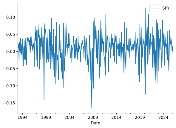
The SPDR S&P 500 ETF Trust (SPY) seeks to track the price and yield performance of the S&P 500 Index before expenses. Figure 2 shows its monthly returns since its 1993 listing.
Practice Problems
These problems apply the chapter’s concepts. Refer to Probability Basics in Stochastic Foundations for Finance for the underlying statistical formulas. Try each problem before expanding its solution.
Problem 1 (Holding-Period Return) Leah Morgan buys a share of Millbrook Properties (MBP), a real estate investment trust, for $50. Over the year the REIT pays $2 in dividends, and Leah sells the share for $53. Compute her capital-gain yield, income yield, and HPR.
Solution
The capital-gain yield is \frac{53 - 50}{50} = 6\%, and the income yield is \frac{2}{50} = 4\%. Thus, \text{HPR} = 6\% + 4\% = 10\%.Problem 2 (Expected Return and Volatility) Felix Brandt is considering shares of Calder Airlines (CAL). Airline profits rise and fall with the economy, and his broker’s research team summarizes CAL’s HPR over the next year as follows.
| State | Probability | HPR |
|---|---|---|
| Boom | 0.25 | 20% |
| Normal | 0.50 | 5% |
| Bust | 0.25 | -10% |
Compute the expected return \mu and the volatility \sigma of CAL.
Solution
\mu = 0.25 \times 0.20 + 0.50 \times 0.05 + 0.25 \times (-0.10) = 0.05 = 5\%. The variance is \sigma^{2} = 0.25 (0.20 - 0.05)^{2} + 0.50 (0.05 - 0.05)^{2} + 0.25 (-0.10 - 0.05)^{2} = 0.01125, so \sigma = \sqrt{0.01125} \approx 0.1061 = 10.61\%.Problem 3 (Annualizing Monthly Statistics) Using several years of data, Hana Ito, an analyst at Ridgecrest Advisors, estimates that Marston Retail’s (MRS) average monthly return is 0.9\% with a monthly standard deviation of 5.5\%. Her reports to clients need annual figures. Treat the annualized arithmetic return as the sum of 12 independent draws from the monthly return distribution. Compute its mean and volatility.
Solution
The annualized arithmetic mean is \bar{r}_{\text{Annual}} = 12 \times 0.9\% = 10.8\%. Volatility scales by the square root of 12, \hat{\sigma}_{\text{Annual}} = \sqrt{12} \times 5.5\% \approx 19.05\%. Because the annualized arithmetic return is the sum of 12 independent monthly returns, its variance scales by 12 and its volatility by \sqrt{12}.Problem 4 (Portfolio Weights and Return) Kofi Mensah has $20,000 to invest. He puts $12,000 in Larkfield Solar (LKS), which returns 8% over the year, and the remaining $8,000 in Bexley Insurance (BXI), which returns -3\%. Compute the portfolio weights w_{LKS} and w_{BXI}, and the portfolio’s HPR.
Solution
The portfolio weights are w_{LKS} = \frac{12{,}000}{20{,}000} = 0.6, \qquad w_{BXI} = \frac{8{,}000}{20{,}000} = 0.4, which sum to one, as they must. Using (1), r_P = 0.6 \times 8\% + 0.4 \times (-3\%) = 3.6\%.Problem 5 (Portfolio Scenario Analysis) Sofia Reyes invests 60% of her savings in Corvel Mining (CVM) and 40% in Dawson Utilities (DWU). The mining company is far more sensitive to the economy than the utility, as the HPR scenarios below show.
| Market | Probability | CVM | DWU |
|---|---|---|---|
| Bull | 0.4 | 25% | 5% |
| Normal | 0.4 | 10% | 8% |
| Bear | 0.2 | -20% | -2% |
Compute the portfolio’s HPR in each state of the market, and then its expected return and standard deviation.
Solution
Using r_{P} = 0.6 \, r_{CVM} + 0.4 \, r_{DWU}, the portfolio’s HPR in each state is
| Market | Probability | Portfolio HPR |
|---|---|---|
| Bull | 0.4 | 17% |
| Normal | 0.4 | 9.2% |
| Bear | 0.2 | -12.8% |
Problem 6 (The Law of One Price and ETF Arbitrage) Late one afternoon, shares of the Harborline Clean Energy ETF (HCE) trade at $24.60, while the net asset value (NAV) of its holdings is $25.00 per share. Daniel Cho works on the ETF desk of Kessler Markets, an Authorized Participant (AP) for HCE. Describe the trade Daniel would execute to profit from the discrepancy, and explain how the trade affects HCE’s price and NAV.
Solution
Since HCE shares are cheap relative to the value of the underlying securities, Daniel buys HCE shares in the open market and delivers them to the ETF issuer in exchange for the underlying securities at NAV. He then sells the underlying securities, which are worth more than what he paid for the ETF shares. Ignoring trading costs, the desk earns about $0.40 per share.
This trade pushes HCE’s market price up, since the AP is buying ETF shares, and pushes down the prices of the underlying securities, since the AP is selling them. Both forces narrow the gap between the ETF’s market price and its NAV, consistent with the law of one price.Problem 7 (Holding-Period Return on a Bond) One year ago, Marisol Vega bought a Penhallow Utilities bond for $980. She received $17 in interest during the year and has just sold the bond for $987. What was her holding-period return?
Solution
The capital-gain yield is \frac{987 - 980}{980} \approx 0.71\%, and the income yield is \frac{17}{980} \approx 1.73\%. Thus, \text{HPR} = \frac{987 - 980 + 17}{980} = \frac{24}{980} \approx 2.45\%.Solution
The expected end-of-year cash flow is \operatorname{E}(CF) = 0.5 \times 70{,}000 + 0.5 \times 200{,}000 = \$135{,}000.
Discounting the expected payoff at 14%, the most Rafael should be willing to pay is P = \frac{135{,}000}{1.14} \approx \$118{,}421.05.
At P = \$118{,}421.05, the portfolio’s expected return is \operatorname{E}(r) = \frac{\operatorname{E}(CF)}{P} - 1 = \frac{135{,}000}{135{,}000 / 1.14} - 1 = 1.14 - 1 = 14\%, which equals the required return by construction.
With a 12% risk premium, the required return rises to 6\%+12\%=18\%, so P = \frac{135{,}000}{1.18} \approx \$114{,}406.78. A higher required risk premium lowers the price of the same expected payoff.
Problem 9 (Mean and Standard Deviation of Stock Returns) Yarrow Biotech (YRB) stock currently trades at $100 and just paid a dividend of $1.80. Nadia Petrova is deciding whether to buy it. Suppose next year’s price and dividend depend on the state of the market as follows:
| State of the Market | Probability | Dividend | Price |
|---|---|---|---|
| Boom | 0.3 | $3 | $120 |
| Normal growth | 0.5 | $2 | $100 |
| Recession | 0.2 | $1 | $80 |
Compute the mean and standard deviation of the returns Nadia can expect from YRB.
Solution
The $1.80 dividend already paid is irrelevant to the investment’s future HPR; only next year’s price and dividend matter. In each state, \text{HPR} = \frac{P_{1} - 100 + D_{1}}{100}.
| State of the Market | Probability | HPR |
|---|---|---|
| Boom | 0.3 | 23% |
| Normal growth | 0.5 | 2% |
| Recession | 0.2 | -19% |