CAPM Anomalies
What Is an Anomaly?
The CAPM makes a sharp prediction: the expected excess return of any asset is its beta times the market risk premium, and nothing else about the asset matters. In the language of the index model, every asset has an alpha of zero once we measure returns relative to the market. An anomaly is a pattern in average returns that the CAPM does not explain: a characteristic of a firm, observable in advance, that predicts its future returns beyond what its beta predicts.
This chapter reviews the main anomalies and measures them with U.S. stock returns. Since the joint-hypothesis problem applies to every one of them, we close by asking what they mean: compensation for risks the CAPM leaves out, mistakes that investors make, or patterns that researchers found by searching too hard.
Testing the CAPM
There are two ways to ask whether the CAPM fits a set of assets. Both start from the excess return R_{i,t} = r_{i,t} - r_{f,t} of asset i in month t.
The time-series test runs, for each asset, the regression of the index model, R_{i,t} = \alpha_{i} + \beta_{i} R_{M,t} + e_{i,t}, \tag{1} and checks whether the intercepts are zero. The CAPM says \alpha_{i} = 0 for every asset. A positive alpha means the asset earned more than its beta justifies.
The cross-sectional test asks whether average returns line up with betas across assets. If we regress the average excess returns \overline{R}_{i} of many assets on their betas, \overline{R}_{i} = \gamma_{0} + \gamma_{1} \beta_{i} + u_{i}, \tag{2} the CAPM predicts an intercept of \gamma_{0} = 0, a slope equal to the market risk premium, \gamma_{1} = \operatorname{E}(R_{M}), and no role for any other characteristic of the assets. The fitted line is the security market line.
Betas are estimated, not observed, and the estimates of individual stock betas are noisy. A regression on noisy betas understates the slope, the classic errors-in-variables problem. Black et al. (1972) addressed it by sorting stocks into ten portfolios on their betas estimated from past returns and then testing the portfolios, whose betas are estimated far more precisely. With NYSE stocks from 1931 to 1965, they found that the time-series intercepts were not zero: low-beta portfolios earned more than the CAPM predicts and high-beta portfolios earned less. The security market line was flatter than the theory says.
Fama and MacBeth (1973) developed the procedure that is now the standard cross-sectional test. Instead of one regression of average returns, run a cross-sectional regression every month, R_{i,t} = \gamma_{0,t} + \gamma_{1,t} \beta_{i} + \gamma_{2,t} z_{i,t-1} + u_{i,t}, \tag{3} where z_{i,t-1} is any other characteristic known before month t. The estimate of each slope is the time-series average of its monthly values, and its standard error comes from the month-to-month variation of those values: \hat{\gamma}_{k} = \frac{1}{T} \sum_{t = 1}^{T} \hat{\gamma}_{k,t}, \qquad t(\hat{\gamma}_{k}) = \frac{\hat{\gamma}_{k}}{s(\hat{\gamma}_{k,t}) / \sqrt{T}}, \tag{4} where s(\hat{\gamma}_{k,t}) is the standard deviation of the T monthly slopes. Each monthly slope is the return on a portfolio, so the t-statistic is the familiar test of whether a portfolio’s average return is zero. For NYSE stocks from 1935 to 1968, Fama and MacBeth could not reject the hypothesis that investors price stocks as if they held mean-variance efficient portfolios: the average slope on beta was positive, while the square of beta and residual risk, which they added as z_{i,t-1}, had no reliable average slope.
Most of the evidence in this chapter uses a simpler tool. Sort stocks into ten portfolios on a characteristic, compute the average excess return of each decile, and compare it with the CAPM’s prediction, \beta_{i} \overline{R}_{M}. If the characteristic is an anomaly, the deciles will drift away from the security market line in a systematic way. The portfolio returns come from Kenneth French’s data library and cover July 1963 to September 2026. Each portfolio is value weighted, and the market is the value-weighted portfolio of all U.S. common stocks.
The Flat Security Market Line
Figure 1 plots the average excess return of the ten beta-sorted portfolios against their betas. The stocks are sorted each June on betas estimated from the previous five years of returns, and the betas on the horizontal axis are estimated over the whole sample with (1).
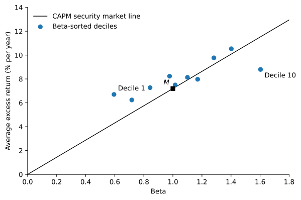
The betas spread out nicely, from 0.59 for the lowest decile to 1.60 for the highest, but average returns barely respond. The lowest-beta decile earned 6.7% a year over the risk-free rate and the highest 8.8%, while the CAPM predicts 4.3% and 11.5%. A portfolio long the lowest-beta decile and short the highest has a CAPM alpha of 5.2% a year, with a t-statistic of 2.10. The finding of Black et al. (1972) has held up for half a century after their sample ended.
A flat security market line does not mean that beta is irrelevant. Black (1972) showed that if investors cannot borrow at the risk-free rate, the CAPM still holds with the risk-free rate replaced by the expected return of a zero-beta portfolio, and the security market line has a higher intercept and a lower slope. An investor who wants more risk than the market and cannot borrow has to buy high-beta stocks instead of levering the market. Frazzini and Pedersen (2014) develop this argument with leverage constraints that differ across investors, and document that high beta comes with low alpha in U.S. stocks, 20 international stock markets, Treasury bonds, corporate bonds and futures. Their betting-against-beta factor holds leveraged low-beta assets and shorts high-beta assets, and it earns significant risk-adjusted returns.
Anomalies in Decile Sorts
Figure 2 applies the same comparison to six other sorts. Each panel plots the average excess return of the ten deciles against the return the CAPM predicts from their betas. Under the CAPM all points lie on the 45-degree line.
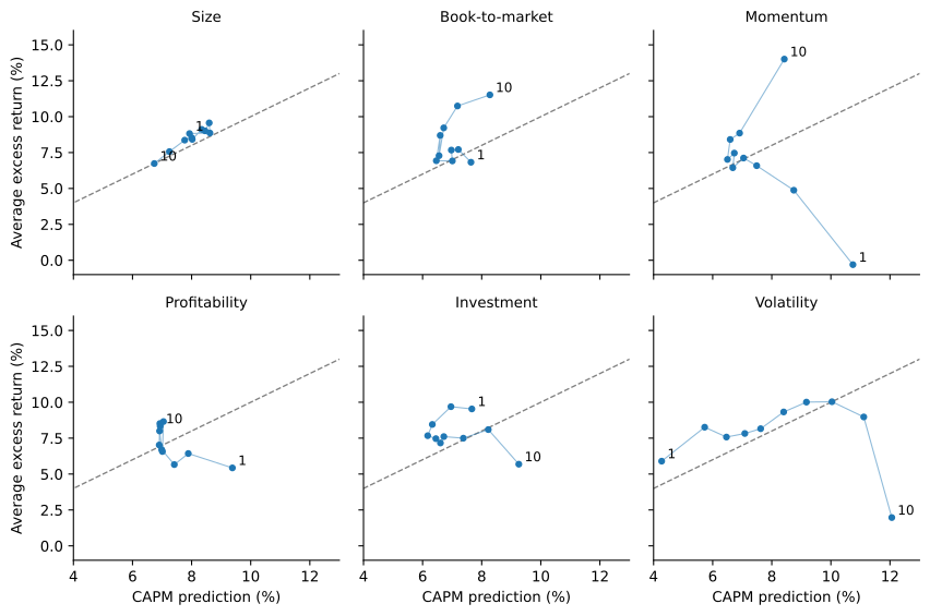
Table 1 summarizes the evidence with one long-short portfolio per sort: it buys the decile the anomaly favors and sells the decile at the other end. The table reports its average return, its beta and its CAPM alpha, all from (1) with the spread as the dependent variable. A long-short portfolio costs nothing to form, so the CAPM predicts that its average return is its beta times the market risk premium.
| Mean (%) | Beta | Alpha (%) | t(alpha) | |
|---|---|---|---|---|
| Small minus big | 2.09 | 0.17 | 0.89 | 0.43 |
| High minus low B/M | 4.69 | 0.09 | 4.05 | 1.88 |
| Low minus high beta | -2.09 | -1.01 | 5.16 | 2.10 |
| Winners minus losers | 14.31 | -0.32 | 16.64 | 5.23 |
| Last month’s losers minus winners | 3.12 | 0.40 | 0.26 | 0.11 |
| Robust minus weak profitability | 2.91 | -0.34 | 5.35 | 3.02 |
| Conservative minus aggressive investment | 3.85 | -0.22 | 5.44 | 3.61 |
| Low minus high accruals | 3.40 | -0.07 | 3.92 | 3.05 |
| Low minus high volatility | 3.93 | -1.08 | 11.72 | 3.93 |
Size
Banz (1981) found that the common stock of small firms, measured by market capitalization, had higher risk-adjusted returns than the stock of large firms in the 1936 to 1975 period. The size effect was the first prominent anomaly. In Figure 2 the size deciles have higher average returns for smaller firms, but they also have higher betas, and since 1963 the CAPM accounts for most of the difference: the small-minus-big spread has an alpha of only 0.9% a year.
The size effect is strongest in the years that Banz studied and weaker since. From July 1926 to December 1980 the smallest decile outperformed the largest by 10.3% a year; from January 1981, the year his paper appeared, to September 2026 the spread averaged -0.9% a year. We return to anomalies that weaken after they are published in a later chapter.
Value
Basu (1977) sorted NYSE industrial firms on their price-earnings ratios from 1957 to 1971 and found that low P/E portfolios earned higher returns than the market, and higher than their risk justified. The ratio of book equity to market equity (B/M) generalizes the idea. A stock with a high B/M is cheap relative to its accounting value, a value stock; a stock with a low B/M is a growth stock. In Figure 2 the high B/M deciles lie above the 45-degree line and the low B/M deciles below it, even though their betas are similar. The high-minus-low spread earns 4.1% a year more than the CAPM predicts.
Beta, Size and Value Together
Fama and French (1992) asked which of these variables matter once all of them are in the same regression. With NYSE, AMEX and Nasdaq stocks from 1963 to 1990, they found that size and B/M capture the cross-sectional variation in average returns associated with beta, size, leverage, B/M and earnings-price ratios. They also found that once the tests allow for variation in beta that is unrelated to size, the relation between beta and average return is flat, even when beta is the only explanatory variable.
We can repeat their test on the CRSP and Compustat data up to December 2025. Their key step deals with the noise in individual betas. Each June, stocks are sorted into ten size deciles, and each size decile is split into ten deciles of beta estimated from the past five years. Every stock then gets the beta of its portfolio among these 100, estimated over the full sample. Because the sort on beta happens within size deciles, the 100 portfolios have betas that vary independently of size. Figure 3 shows the result: within each size group, average returns do not rise with beta. Across size groups, smaller firms have both higher betas and higher returns, which is what makes beta look priced when size is left out.
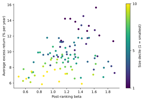
Table 2 reports the Fama-MacBeth slopes of (4) for July 1963 to December 2025, with an average of 2,786 stocks a month. The size variable is the logarithm of market equity, \ln(ME), and the value variable is \ln(BE/ME).
| Beta | \ln(ME) | \ln(BE/ME) | |
|---|---|---|---|
| Beta alone | 0.19 (0.81) | ||
| Size alone | -0.11 (-3.15) | ||
| Book-to-market alone | 0.33 (6.33) | ||
| Beta and size | -0.15 (-0.68) | -0.13 (-3.88) | |
| Beta, size and book-to-market | -0.02 (-0.12) | -0.09 (-2.53) | 0.24 (4.89) |
The pattern matches what Fama and French (1992) found for their earlier sample. On its own, beta has an average slope of 0.19% a month with a t-statistic of only 0.81, so we cannot reject that beta earns nothing at all. Size and book-to-market are both significant, alone or together, and adding them pushes the slope on beta to essentially zero.
Momentum and Reversal
Jegadeesh and Titman (1993) showed that strategies that buy stocks that did well over the past 3 to 12 months and sell stocks that did poorly earn significant positive returns over the following 3 to 12 months. In their 1965 to 1989 sample, a strategy that ranks stocks on their past six months of returns earns about 1% a month whatever the holding period. The momentum deciles in Figure 2 rank stocks on their returns from 12 months to 2 months before portfolio formation, skipping the most recent month. Past losers have higher betas than past winners in this sample, so the CAPM makes the anomaly larger rather than smaller: the winners-minus-losers spread has a beta of -0.32 and an alpha of 16.6% a year, with a t-statistic of 5.23, the largest in Table 1.
The most recent month is skipped because returns over one month tend to reverse. Jegadeesh (1990) found highly significant negative first-order serial correlation in monthly stock returns. The short-term reversal spread in Table 1 buys last month’s losers and sells last month’s winners. Its average return of 3.1% a year is mostly compensation for market risk: its alpha is 0.3% a year in these value-weighted portfolios.
Profitability, Investment and Accruals
Three more anomalies come from accounting data. Novy-Marx (2013) showed that profitability, measured by gross profits relative to assets, has roughly the same power as B/M in predicting the cross-section of average returns, and that profitable firms earn significantly higher returns despite their higher valuation ratios. Titman et al. (2004) found that firms that substantially increase their capital investments subsequently earn negative benchmark-adjusted returns. Sloan (1996) found that the accrual component of earnings persists less than the cash-flow component, but that stock prices behave as if investors fixate on earnings and fail to tell the two apart, so firms with high accruals subsequently earn lower returns.
The profitability and investment deciles in Figure 2 use the operating profitability and asset growth measures of the Fama-French five-factor model, which Beyond the CAPM takes up. Both produce large alphas in Table 1, and so does the sort on accruals.
Volatility
Ang et al. (2006) found that stocks with high idiosyncratic volatility, measured relative to the Fama-French three-factor model, have low average returns: from July 1963 to December 2000 the difference between the highest and lowest quintiles was -1.06\% a month. The volatility deciles in Figure 2 sort on the total variance of daily returns over the previous 60 days. The highest-volatility decile has the highest beta and the lowest average return, which places it far below the 45-degree line. The low-minus-high volatility spread has the largest negative beta in Table 1, -1.08, which raises its CAPM alpha to 11.7% a year. This anomaly is a close relative of the flat security market line: high-volatility stocks are also high-beta stocks.
Long-Short Returns over Time
The averages in Table 1 hide large swings. Figure 4 shows what $1 invested in Treasury bills plus each long-short spread would have grown to, against $1 invested in the market. A zero-cost spread can be added to any portfolio, so holding T-bills plus the spread is a self-financing strategy with the same risk as the spread.
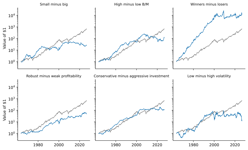
Two features stand out. First, several anomalies were much stronger in some decades than in others: the value spread had its best years from 2000 to 2006, peaked in mid-2007, and has lost money on average since. Second, momentum, the strategy with the largest average return, also suffered the largest loss. Its collapse in 2009 came when the stocks that had fallen most during the financial crisis, the past losers it was short, rebounded with the market. An anomaly can have a large alpha and still be a risky strategy to follow.
Before and After Publication
A pattern found by chance has no reason to continue after the sample in which it was found. A pattern that reflects mispricing may shrink once it is published and investors trade on it. Either way, the years after publication are a test that the original authors could not have fitted. Figure 5 splits each spread in Table 1 at the year the study cited above was published, and estimates its CAPM alpha before and after. Our data start in July 1963, so the period before publication covers only part of each original sample, and for beta only about 10 years.
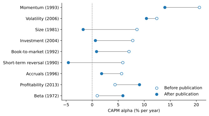
Most anomalies weakened. The average alpha of the nine spreads fell from 8.2% a year before publication to 4.0% after. Size, book-to-market, short-term reversal, investment and accruals all have alphas after publication that are small or negative, with t-statistics below 0.9. Momentum kept an alpha of 14.0% a year (t = 2.69), and low volatility one of 10.4% (t = 1.69). Two spreads went the other way. The low-beta spread earned more after 1972 than in the short period before it, and profitability has had a larger alpha since 2013, though over only about 13 years. McLean and Pontiff (2016) find the same decline across 97 published predictors, and Limits to Arbitrage takes up what it says about chance findings and arbitrage.
Risk, Mispricing or Data Mining?
Every anomaly in this chapter is a rejection of the joint hypothesis that markets are efficient and that the CAPM describes expected returns. There are three broad ways to read the evidence.
Missing risk factors. The CAPM may be the wrong model of risk. Fama and French (1993) proposed a three-factor model that adds a size factor and a value factor to the market, and Fama and French (1996) found that, except for the continuation of short-term returns, the anomalies known at the time largely disappear in that model. They interpret the results as consistent with rational asset pricing in Merton’s intertemporal CAPM or Ross’s APT, with size and value standing in for undiversifiable risks such as relative distress. Beyond the CAPM develops these models.
Mispricing. Lakonishok et al. (1994) argue that value strategies earn higher returns because they exploit the suboptimal behavior of the typical investor, who extrapolates past growth too far into the future, and not because value stocks are fundamentally riskier. Daniel and Titman (1997) found that it is the characteristics, size and B/M themselves, rather than the comovement of returns with factors, that explain the cross-sectional variation in returns, which is harder to square with a risk explanation. The explanations offered for momentum and accruals in the original papers, slow reaction to information and fixation on reported earnings, are also behavioral. If prices are wrong, the question becomes why arbitrageurs do not correct them, the subject of Limits to Arbitrage.
Data mining. Researchers have tested hundreds of characteristics, and some will look significant by chance. Harvey et al. (2016) argue that once we account for this multiple testing, a newly proposed factor needs a t-statistic greater than 3.0, not the usual 2.0. Most of the spreads in Table 1 clear that bar over the full sample, but Figure 5 shows that for many of them the alpha came before publication. A decline after publication is consistent with a chance finding, with a premium that investors competed away once it was known, or with both. The anomalies that kept their alphas for decades after publication, momentum and low volatility above all, are the strongest evidence against data mining.
Practice Problems
These problems give you a chance to practice the concepts introduced in this chapter. Try to solve each one on your own before expanding the solution.
Problem 1 (Reading a Decile Sort) Priya Raman, an analyst at Westerly Advisors, sorts stocks into deciles on book-to-market. Over her sample the market risk premium averaged 6\% a year. For the two extreme deciles she finds:
| Portfolio | Average Excess Return | Beta |
|---|---|---|
| Decile 1 (low B/M) | 6.5% | 1.05 |
| Decile 10 (high B/M) | 11.0% | 1.15 |
- Compute the excess return the CAPM predicts for each decile and its alpha.
- Priya forms a portfolio that is long decile 10 and short decile 1. What are its average return, its beta and its alpha?
- Can the higher beta of value stocks explain why they earned more?
Solution
The CAPM predicts 1.05 \times 6\% = 6.3\% for decile 1 and 1.15 \times 6\% = 6.9\% for decile 10. The alphas are 6.5\% - 6.3\% = 0.2\% and 11.0\% - 6.9\% = 4.1\%.
The spread earns 11.0\% - 6.5\% = 4.5\% and has a beta of 1.15 - 1.05 = 0.10. Its alpha is 4.5\% - 0.10 \times 6\% = 3.9\%, which equals the difference between the two alphas, 4.1\% - 0.2\%.
No. The difference in betas accounts for only 0.6\% of the 4.5\% difference in average returns. The rest is the alpha that makes book-to-market an anomaly.
Problem 2 (Fama-MacBeth by Hand) A cross-sectional regression of stock excess returns on beta, run separately in six months, gives the following slopes on beta, in percent: 0.8, -1.2, 0.5, 1.6, -0.9 and 0.4.
- Compute the Fama-MacBeth estimate of the slope on beta and its t-statistic.
- If the slopes kept the same mean and standard deviation, how many months of data would we need for a t-statistic of 2?
- Why does the Fama-MacBeth procedure use the variation of the monthly slopes, rather than the standard errors of the monthly regressions, to measure precision?
Solution
The average slope is (0.8 - 1.2 + 0.5 + 1.6 - 0.9 + 0.4)/6 = 1.2/6 = 0.2\%. The deviations from the mean are 0.6, -1.4, 0.3, 1.4, -1.1 and 0.2, whose squares add up to 5.62, so the standard deviation is \sqrt{5.62/5} = 1.060\%. The t-statistic is 0.2/(1.060/\sqrt{6}) = 0.2/0.433 = 0.46.
We need 0.2/(1.060/\sqrt{T}) = 2, or \sqrt{T} = 2 \times 1.060/0.2 = 10.6, so T = 112.4, about 113 months or more than nine years.
Stock returns in the same month are correlated, because they all respond to the same news. The standard errors of a single cross-sectional regression treat the stocks as independent observations and understate the uncertainty. Each monthly slope is the return on a portfolio, and the variation of that return from month to month includes the effect of common shocks.
Problem 3 (Leverage and the Flat Security Market Line) A stylized version of the beta deciles has a low-beta portfolio L with beta 0.6 and average excess return 6.7\%, and a high-beta portfolio H with beta 1.6 and average excess return 8.8\%. Marcus Bell wants a portfolio with a beta of 1.6.
- What excess return does Marcus expect if he buys H?
- What excess return does he expect if he instead invests in L and borrows at the risk-free rate to reach a beta of 1.6?
- Redo the previous part if Marcus can only borrow at 2\% above the risk-free rate.
- Why might the security market line be flat if many investors cannot borrow?
Solution
8.8\%.
He needs a weight of w = 1.6/0.6 = 2.667 in L, financed by borrowing 1.667 times his wealth. His expected excess return is 2.667 \times 6.7\% = 17.9\%.
The borrowing costs 2\% over the risk-free rate on 1.667 times his wealth, so the expected excess return falls to 17.9\% - 1.667 \times 2\% = 14.5\%, still well above what H offers.
Investors who want more risk than the market but cannot borrow, or face a high borrowing rate, reach for risk by buying high-beta stocks. Their demand raises the prices of high-beta stocks and lowers their expected returns, while low-beta stocks are left cheap. This is the zero-beta argument of Black (1972) and the leverage-constraint argument of Frazzini and Pedersen (2014). Note that leverage also scales up the firm-specific risk of L, so the levered position is more volatile than its beta alone suggests.
Problem 4 (How Many False Discoveries?) A group of researchers tests 300 firm characteristics as predictors of returns. Suppose none of them truly predicts returns, and the tests are independent.
- How many characteristics do they expect to find significant with the usual cutoff |t| > 1.96?
- How many do they expect with the cutoff |t| > 3.0 proposed by Harvey et al. (2016)? The two-sided probability that a standard normal exceeds 3 in absolute value is 0.27\%.
- Why is evidence from a sample that starts after the original study ended more convincing than a higher t-statistic in the original sample?
Solution
Each test has a 5\% chance of a false rejection, so they expect 300 \times 0.05 = 15 false discoveries.
300 \times 0.0027 = 0.81, less than one false discovery.
A higher cutoff guards against chance findings only if we know how many tests were run, which includes the tests that were never reported. Returns from a new sample were not available when the characteristic was chosen, so the researchers could not have searched over them. If the pattern was a chance finding, it should disappear out of sample.
Problem 5 (Did the Size Effect Disappear?) A small-minus-big portfolio earned an average of 0.80\% a month with a monthly standard deviation of 6.0\% over the 660 months from 1926 to 1980. Over the next 540 months it averaged -0.05\% a month with a standard deviation of 4.0\%.
- Compute the t-statistic of the average return in each period.
- Test whether the average return differs between the two periods, treating the periods as independent samples.
- Give two explanations for the change.
Solution
The standard errors are 6.0/\sqrt{660} = 0.234\% and 4.0/\sqrt{540} = 0.172\%. The t-statistics are 0.80/0.234 = 3.43 and -0.05/0.172 = -0.29.
The difference is 0.85\% with a standard error of \sqrt{0.234^{2} + 0.172^{2}} = 0.290\%, so t = 0.85/0.290 = 2.93. The average return was significantly lower in the second period.
The original finding may have been partly due to chance, a pattern that happened to hold in the period researchers looked at. Alternatively, the premium may have been real but competed away once it was published, as investors bought small stocks and raised their prices.
Problem 6 (The Alpha of Momentum) A winners-minus-losers portfolio earns an average of 1.2\% a month and has a market beta of -0.3. The market risk premium is 0.5\% a month.
- Compute the CAPM alpha of the strategy.
- Explain why a negative beta makes the alpha larger than the average return.
- In one month after a market crash, the market excess return is +20\%. How much does the strategy’s market exposure alone contribute to its return that month? Why does this matter for an investor following the strategy?
Solution
\alpha = 1.2\% - (-0.3)(0.5\%) = 1.35\% a month.
A negative beta means the strategy is a partial hedge against market risk. The CAPM says a hedge should earn less than the risk-free rate, so any positive return counts as abnormal, and the alpha exceeds the average return by 0.3 \times 0.5\% = 0.15\%.
The market exposure contributes -0.3 \times 20\% = -6\%. After a crash the past losers are the stocks that fell the most, often high-beta stocks, so the strategy’s beta becomes strongly negative just when the market is most likely to rebound sharply. The average alpha comes with the risk of a large loss in a single month, as in 2009 in Figure 4.