Limits to Arbitrage and Investor Anomalies
The efficient markets argument has two steps. Some investors may be irrational, but rational arbitrageurs will trade against them, and their trading will push prices back to fundamental values. Investors who keep buying overpriced assets will lose money to the arbitrageurs and eventually leave the market. CAPM Anomalies and Beyond the CAPM documented patterns in returns that the CAPM, and sometimes any factor model, cannot explain. If some of these patterns are mispricing, the second step of the argument must fail somewhere. This chapter asks why arbitrage may not correct prices, looks at cases where mispricing is beyond doubt, and then turns to the evidence on how individual investors actually behave.
What Arbitrage Requires
An arbitrage in the textbook sense needs no capital and carries no risk. Most of what traders call arbitrage is different: buy a security that looks cheap, sell a close substitute that looks expensive, and wait for the prices to converge. Barberis and Thaler (2003) summarize why such trades can be risky and costly even when the mispricing is large.
- Fundamental risk. Substitutes are rarely perfect. An arbitrageur who buys an undervalued stock and shorts other stocks in its industry to hedge is still exposed to news about the company itself.
- Noise trader risk. The mispricing can get worse before it gets better. The investors whose demand pushed the price away from fundamental value may push it further.
- Implementation costs. Commissions, bid-ask spreads and price impact, and above all the cost of shorting: borrowing fees, the risk that the lender recalls the shares, and rules that forbid many institutions from shorting at all.
The logic of the efficient markets hypothesis runs in one direction. If prices are right, there is no free lunch: no strategy earns a return in excess of its risk without cost. The reverse does not follow. The absence of a free lunch does not mean that prices are right, because a mispricing that is risky or costly to exploit is not a free lunch either.
Pontiff (2006) argues that the most important cost is idiosyncratic risk. Systematic risk can be hedged with index futures or other stocks, but the risk specific to the mispriced security cannot. A risk-averse arbitrageur who expects an abnormal return \alpha on a security with idiosyncratic variance \sigma^{2}(e) takes a position proportional to \alpha / \sigma^{2}(e). This is exactly the weight of a security in the active portfolio of the Treynor-Black model. Large idiosyncratic risk keeps the position small, so the mispricing survives. Pontiff surveys evidence that idiosyncratic risk explains more of the mispricing that survives than transaction costs do.
Noise Trader Risk
De Long et al. (1990) showed that noise trader risk alone can keep prices away from fundamental values, even for an asset with no fundamental risk at all. In their model, investors live for two periods and choose a portfolio when young. There are two assets that pay the same dividend r every period. The safe asset is in unlimited supply, so its price is always one. The unsafe asset is in fixed supply, so its price is set by demand. Since the two assets pay the same dividends, the fundamental value of the unsafe asset is also one.
A fraction \mu of the young are noise traders, who misperceive the expected price of the unsafe asset next period by \rho_{t}. Their misperception is random and independent over time, normal with mean \rho^{*} and variance \sigma_{\rho}^{2}. The rest are sophisticated investors, who know the true distribution of prices. Both types have constant absolute risk aversion \gamma. In the steady state, the price of the unsafe asset is p_{t} = 1 + \frac{\mu (\rho_{t} - \rho^{*})}{1 + r} + \frac{\mu \rho^{*}}{r} - \frac{2 \gamma \mu^{2} \sigma_{\rho}^{2}}{r (1 + r)^{2}}. \tag{1} The second term moves the price with the current mood of noise traders. The third is the average effect of their optimism or pessimism. The last term is the heart of the model. Sophisticated investors who buy the unsafe asset when noise traders are pessimistic face the risk that noise traders will be even more pessimistic when the time comes to sell. That risk exists only because noise traders exist, and sophisticated investors require compensation for bearing it, so the price is lower than the fundamental value on average. Noise traders “create their own space”: an asset with no fundamental risk becomes risky, and earns a premium, because of them.
The model also challenges the second step of the efficient markets argument, that irrational investors lose money and disappear. Noise traders who are on average optimistic hold more of the unsafe asset, so they earn more of its risk premium, a premium they themselves create. Against that, they buy at high prices and sell at low ones, and their own demand lowers the premium they earn. For moderate optimism, the first effects win and noise traders earn higher expected returns than sophisticated investors. They still have lower expected utility, because they bear more risk than they think, and higher expected returns are not the same as long-run survival: a noise trader’s wealth is also more volatile. What the model shows is that the claim that irrational investors must lose money is not true in general.
Performance-Based Arbitrage
In practice, arbitrage is done by specialists who manage other people’s money. Shleifer and Vishny (1997) pointed out that this separates the brains from the capital. Investors cannot judge whether an arbitrageur’s strategy is sound, so they judge it by its returns, and they withdraw money after losses. Shleifer and Vishny call this performance-based arbitrage.
Their model has three dates. A stock has fundamental value V, which becomes known at the last date. Noise traders are pessimistic and depress the price by S_{t} at dates 1 and 2. Arbitrageurs have funds F_{1} at date 1, invest D_{1} of them in the stock, and the price is p_{1} = V - S_{1} + D_{1}. If noise traders become more pessimistic at date 2, the price falls and the arbitrageurs lose money. Their investors respond by withdrawing funds, so that F_{2} = F_{1} - a D_{1} \left( 1 - \frac{p_{2}}{p_{1}} \right) \qquad p_{2} = V - S_{2} + F_{2}, \tag{2} where a measures how strongly funds respond to performance. With a = 1 the arbitrageurs simply lose the money they lost on the trade. With a > 1 investors also take money out. Arbitrageurs are then forced to sell exactly when the mispricing is largest and their expected return is highest, and their selling pushes the price down further.
Skill versus Luck measured how mutual fund flows respond to past returns. Money chases the best funds, but investors leave the worst funds only slowly, so for mutual funds a is small after losses. The mechanism bites harder for hedge funds, whose investors can redeem after a bad quarter, and for any leveraged arbitrageur, whose lenders demand more collateral as the position loses money.
Example 1 (Arbitrageurs Forced to Sell) Let V = 1, F_{1} = 0.2, S_{1} = 0.3 and a = 1.2. Arbitrageurs invest all their funds at date 1, so D_{1} = 0.2 and p_{1} = 1 - 0.3 + 0.2 = 0.9. At date 2 noise trader pessimism deepens to S_{2} = 0.4.
By (2), F_{2} = 0.2 - 1.2 \times 0.2 \times (1 - p_{2} / 0.9) and p_{2} = 0.6 + F_{2}. Substituting the first equation into the second gives p_{2} = 0.56 + 0.2667 \, p_{2}, so p_{2} = 0.7636 and F_{2} = 0.1636. The arbitrageurs’ capital fell by nearly a fifth, 0.0364, partly from losses and partly from withdrawals, on a position that will pay off at date 3, and the price is 0.2364 below fundamental value. If the fund’s capital did not respond to its returns at all, a = 0, the arbitrageurs would still have 0.2 to invest and the price would be 0.8. Losses and withdrawals together deepen the mispricing by 0.0364.
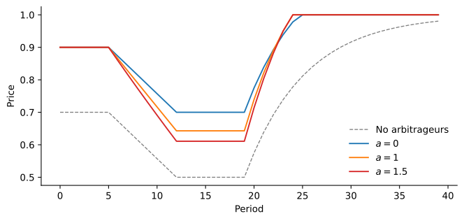
Figure 1 extends the example to many periods. Noise trader pessimism rises from 0.3 to 0.5, stays there for a while, and then fades. With a = 0, the fund’s capital does not respond to its returns, as if investors replaced every loss, the arbitrageurs keep buying, and the price falls to 0.70. With a = 1, the arbitrageurs lose money as the price falls, and the price falls to 0.64. With a = 1.5, investors also withdraw money, and the price falls to 0.61. In every case, the price returns to fundamental value once pessimism fades, and the arbitrageurs who stayed in earn large returns. The ones who were forced out do not.
Shleifer and Vishny drew several predictions from this argument. Arbitrage resources are concentrated in markets where the risk of a trade can be hedged and the trade converges quickly, such as bonds and currencies, and less in stocks, where mispricing is harder to identify and to hedge. And mispricing should be largest in securities with high idiosyncratic volatility, which arbitrageurs cannot hedge. A year after the paper appeared, the hedge fund Long-Term Capital Management became the best-known illustration. Its convergence trades moved against it during the Russian default crisis of 1998, its capital shrank, and a consortium of its lenders, organized by the Federal Reserve Bank of New York, took it over.
Riding Bubbles
The arguments so far explain why arbitrageurs may fail to correct a mispricing. Abreu and Brunnermeier (2003) showed that they may also choose to make it worse. In their model, a stock’s price rises above its fundamental value, and rational arbitrageurs learn of the overpricing one by one, at random times. Together they could correct it by selling, but no one knows how many others have noticed. An arbitrageur who sells too early gives up the gains of a rising price, while one who sells just before the others captures them. The equilibrium is to ride the bubble for a while and sell only when the chance of a crash in the near future becomes high enough. The bubble can then last long after every arbitrageur knows that the price is too high, and news that lets arbitrageurs coordinate can trigger a crash out of proportion to the news itself.
Brunnermeier and Nagel (2004) found that this is what hedge funds did during the technology bubble. From their quarterly holdings, hedge funds held more technology stocks than the market portfolio throughout the bubble: by March 2000, when prices peaked, technology stocks made up 31% of hedge fund stock portfolios against 21% of the market. They cut their holdings of individual stocks before those stocks’ prices peaked and, on average, earned abnormal returns on them. The fund managers who tried to fight the bubble fared worse. Julian Robertson’s Tiger Fund refused to buy technology stocks, lost about a quarter of its assets to withdrawals in the last quarter of 1999, and announced its liquidation in March 2000, just as prices began to fall. George Soros’s Quantum Fund, which raised the share of its portfolio in technology stocks from less than 20% to about 60% in 1999, suffered mounting losses when prices fell, and its manager, Stanley Druckenmiller, resigned in April 2000. Being right about fundamental value is not enough. Timing matters, and an arbitrageur who is early can be out of business before being proved right.
Short-Sale Constraints
Many anomalies are concentrated in overpriced stocks, the short side of the trade. Miller (1977) explained why short-sale constraints matter. If investors disagree about a stock’s value and few of them can sell short, the stock is held by the most optimistic investors, and its price reflects their valuation rather than the average one. The more investors disagree, the higher the price relative to the average valuation. Without short sales, the pessimists’ views have no effect on the price. Miller noted that this could explain the low returns of risky stocks and new issues. The same argument does not work in reverse: investors who think a stock is cheap can simply buy it, so short-sale constraints make overpricing more common than underpricing.
To short a stock, an investor borrows it from a lender, usually an institution, and pays a fee. D’Avolio (2002) studied 18 months of data from a large lender, from 2000 to 2001. For most stocks shorting is cheap: 91% of the stocks on loan cost less than 1% a year to borrow, and most cost about 0.15%. About 9% of stocks were “special”, with fees averaging 4.3% a year, and a few reached extreme levels: 50% a year for Krispy Kreme, and 35% for Palm in July 2000. Special stocks are small, have half the institutional ownership of other stocks and twice the dispersion of analysts’ forecasts, and loan fees rise with share turnover, a sign of disagreement among investors, just as Miller’s argument suggests. D’Avolio concluded that borrowing costs are too low on average to explain the return anomalies, but can be prohibitive in exactly the stocks where disagreement is greatest.
Mispricing That Survives
The difficulty in testing for mispricing is that we rarely know the fundamental value of a stock. There are a few cases, though, in which we know the relation between two prices exactly. They make it possible to see mispricing without any model of risk.
Twin Shares
In 1907, Royal Dutch Petroleum and Shell Transport and Trading merged their interests on a 60:40 basis while remaining separate companies. Royal Dutch had a claim to 60% of the cash flows of the combined group and Shell to 40%, so the market value of Royal Dutch should always have been 1.5 times the market value of Shell. Royal Dutch traded mostly in Amsterdam and New York, Shell mostly in London. Froot and Dabora (1999) studied this and two other twin-share companies from 1980 to 1995. The deviations from parity were large and persistent, 30% or more, and the relative price moved with the markets where each stock mainly traded: when the U.S. market rose relative to the U.K. market, Royal Dutch rose relative to Shell. The location of trade affected prices, even though the cash flows were fixed by contract.
Figure 2 shows the deviation from parity for the U.S. listings of the two companies. Royal Dutch was 31% below parity in June 1981 and 24% above it in October 1998. The deviations narrowed only in the early 2000s, and the companies unified in 2005.
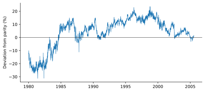
The arbitrage seems simple: buy the cheap twin, short the expensive one, and wait. The position has no fundamental risk, since the two stocks are claims on the same cash flows. But it has no date at which the prices must converge, so it is exposed to noise trader risk in its purest form. An arbitrageur who bought Royal Dutch when it was 10% below parity in March 1983 saw it fall further over the next six months, and the deviation lasted for years. Long-Term Capital Management was among the hedge funds that took this position.
Carve-Outs
Lamont and Thaler (2003) studied an even starker case. On March 2, 2000, 3Com sold about 5% of its subsidiary Palm, the maker of handheld computers, in an initial public offering. It kept the other 95% and announced that it would distribute those shares to its own shareholders within a few months, at about 1.525 Palm shares per 3Com share. A share of 3Com was therefore worth at least 1.525 Palm shares, plus whatever 3Com’s other businesses, cash and securities were worth. That other value is the stub: \text{stub} = P_{\text{3Com}} - 1.525 \, P_{\text{Palm}}. \tag{3}
At the end of the first day of trading, Palm closed at $95.06 and 3Com at $81.81, so the stub was -$63.16 per share: by (3), the market valued 3Com’s businesses outside Palm at about -\$22 billion. Figure 3 shows that the stub stayed negative for two months. It turned positive on May 9, after the tax ruling and the date of the distribution were announced, and the distribution took place at the end of July.
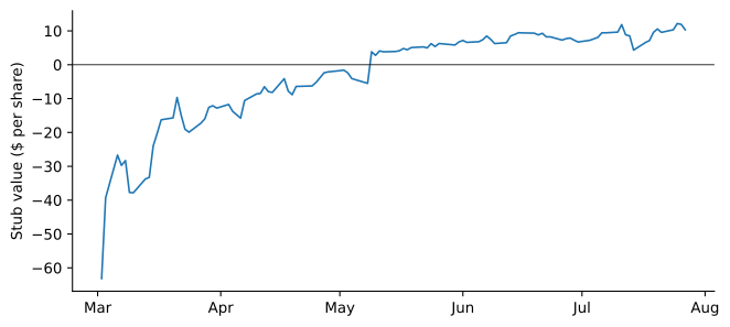
The arbitrage is to buy 3Com and short 1.525 Palm shares. It would have been profitable, but it was hard to do. With only 5% of Palm’s shares in public hands, few were available to borrow, and so many investors tried that short interest in Palm reached 147.6% of the shares outstanding at its peak, as shares lent out were bought by others and lent out again. Borrowing fees were high, and the prices of Palm options implied that shorting Palm cost far more than shorting a normal stock. Lamont and Thaler called the episode “not an exploitable arbitrage opportunity” but “a case of blatant mispricing”. Two things are needed for such mispricing: investors willing to pay too much, and costs that keep arbitrageurs from correcting the price.
Mitchell et al. (2002) studied 82 cases from 1985 to 2000 in which a parent company’s market value was less than the value of its stake in a publicly traded subsidiary. These trades carry real risks. In about 30% of cases the link between the two prices was broken before the mispricing disappeared, most often because the parent or the subsidiary was acquired. The time to convergence was uncertain, with a median of 92 days and some cases lasting years, and the mispricing often widened along the way. Arbitrageurs who had to post enough collateral to avoid margin calls would have earned much lower returns than those who could hold the positions with borrowed money.
Where Arbitrage Is Costly
If limits to arbitrage allow mispricing to persist, mispricing should be largest where arbitrage is hardest. Baker and Wurgler (2006) built an index of investor sentiment from measures such as the closed-end fund discount, the number of initial public offerings and their first-day returns, and trading volume. When sentiment was high, small, young, unprofitable, highly volatile and non-dividend-paying stocks earned low subsequent returns relative to other stocks, and when sentiment was low the pattern weakened or reversed. These are the stocks that are hardest to value and hardest to arbitrage.
Stambaugh et al. (2012) combined this index with eleven anomalies, including momentum, profitability, asset growth and net stock issues. Each anomaly earned larger returns after periods of high sentiment, and almost all of the difference came from the short leg, the stocks the anomaly says are overpriced. The long leg earned about the same after high and low sentiment. This is what Miller’s argument predicts: when sentiment is high, some stocks become overpriced, and short-sale constraints keep arbitrageurs from correcting them. Underpricing does not need short sales to be corrected.
Anomalies after Publication
CAPM Anomalies split nine decile spreads at the year their anomaly was published. McLean and Pontiff (2016) looked at 97 predictors of stock returns from published academic studies. If the original findings were statistical flukes, the predictors should stop working right after the original sample period. If they were mispricing that arbitrageurs did not know about, they should weaken after publication, once arbitrageurs learned of them. The returns of the long-short portfolios were 26% lower after the end of the original sample period but before publication, a decline that sets an upper bound on how much of the original returns was a statistical fluke. After publication the returns were 58% lower. The difference, about 32%, is the effect of publication. The decline was larger for predictors concentrated in liquid stocks with low idiosyncratic risk, which are cheaper to arbitrage, and trading volume and short interest in the predictor portfolios rose after publication.
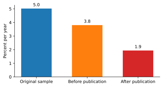
We can repeat the exercise with the factors of Jensen et al. (2023), whose documentation records, for each factor, the original study and its sample period. Of the 142 factors that can be traced to a single study, 77 had t-statistics above 1.96 in their original sample period, in our data. Figure 4 shows their average returns in three periods. Returns fall by 24% after the end of the original sample and by 61% after publication, close to the 26% and 58% of McLean and Pontiff. The anomalies did not disappear, though. After publication the average factor still earned 1.9% a year, and among the decile spreads, momentum and low volatility kept large alphas for decades after they were published.
Investor Anomalies
Limits to arbitrage explain why mispricing can survive, but not where it comes from. For that we need investors whose demand does not follow fundamental value, and whose errors are shared widely enough not to cancel out. A large body of evidence, much of it from the trading records of individual investors, documents systematic patterns in how people invest. Barberis and Thaler (2003) survey the psychology behind them: overconfidence in one’s own judgment, the tendency to read too much into short samples, anchoring on irrelevant numbers, and preferences that depart from expected utility.
Prospect Theory
Kahneman and Tversky (1979) gave subjects choices between hypothetical gambles and found systematic violations of expected utility theory. In one pair of problems, 82% of subjects preferred 2,400 for sure to a gamble paying 2,500 with probability 0.33, 2,400 with probability 0.66 and nothing with probability 0.01. But 83% preferred 2,500 with probability 0.33 to 2,400 with probability 0.34. The second pair is the first with a 0.66 chance of 2,400 removed from both options, so expected utility theory says the preferences should be the same. People give extra weight to outcomes that are certain. When the same gambles were posed as losses, preferences reversed: subjects preferred a 0.80 chance of losing 4,000 to a sure loss of 3,000.
Kahneman and Tversky proposed a theory with three features. People evaluate outcomes as gains and losses relative to a reference point, not as levels of final wealth. The value function is concave for gains and convex for losses, so people are risk averse over gains and risk seeking over losses. And it is steeper for losses than for gains: in their words, “the aggravation that one experiences in losing a sum of money appears to be greater than the pleasure associated with gaining the same amount.” Probabilities enter through decision weights, which overweight small probabilities.
The Disposition Effect
Prospect theory predicts that investors who measure gains and losses from the price they paid will sell winners too early and hold losers too long. A stock that has gained puts the investor in the concave region, where a sure gain is attractive. A stock that has lost puts the investor in the convex region, where holding on in the hope of breaking even is attractive. Odean (1998) tested this with the trading records of 10,000 accounts at a large discount broker from 1987 to 1993. On each day an investor sold a stock, he counted every stock in the portfolio as a realized gain or loss if it was sold, and as a paper gain or loss if it was held, by comparing its price with its average purchase price. The proportions of gains and losses realized are \text{PGR} = \frac{\text{realized gains}}{\text{realized gains} + \text{paper gains}} \qquad \text{PLR} = \frac{\text{realized losses}}{\text{realized losses} + \text{paper losses}}. \tag{4} Over the whole year PGR was 0.148 and PLR was 0.098: a stock that was up was about 50% more likely to be sold than a stock that was down. Taxes favor the opposite, since realizing losses reduces taxes, and in December, when the tax year ends, investors did realize losses at a higher rate than gains. Selling winners did not pay off either. Over the following year, the winners investors sold beat the market by 3.4 percentage points more than the losers they kept.
Overconfidence and Trading
Barber and Odean (2000) studied 66,465 households at the same kind of broker from 1991 to 1996. The average household turned over 75% of its portfolio each year. The households that traded most earned about the same gross returns as the others, but after commissions and spreads their net return was 11.4% a year, while the market returned 17.9%. Their explanation is overconfidence: investors who overestimate the precision of their information trade too much. Overconfidence is hard to measure directly, so in a second paper Barber and Odean (2001) used gender as a proxy, since psychologists find that in areas such as finance men are more overconfident than women. Men traded 45% more than women, and trading reduced their net returns by 2.65 percentage points a year, against 1.72 for women. Single men traded 67% more than single women.
Attention
There are thousands of stocks to buy, but an investor can only sell what is already in the portfolio. Barber and Odean (2008) argued that individual investors therefore buy the stocks that catch their attention. Individuals were net buyers of stocks with unusually high trading volume, extreme returns on the previous day, or news, while institutional investors showed the opposite pattern. Barber et al. (2022) studied the users of Robinhood, a trading app that attracted many new investors. On days when the number of Robinhood users holding a stock jumped the most, those stocks had large returns on the same day and abnormal returns of about -4.7\% over the following 20 trading days. The more extreme the herding, the larger the subsequent loss.
Diversification Mistakes
French and Poterba (1991) found that at the end of the 1980s, U.S. investors held 93.8% of their stock portfolios in U.S. stocks, Japanese investors 98.1% in Japanese stocks and British investors 82% in British stocks. To justify these portfolios with mean-variance reasoning, investors in each country would have to expect domestic stocks to earn several percentage points a year more than foreign ones, more than 500 basis points in the case of British investors. They concluded that the lack of diversification is the result of investor choices, not of legal or institutional barriers.
Benartzi and Thaler (2001) found that people often diversify by splitting money evenly among the options they are offered. In their experiments, employees asked to divide retirement savings between a stock fund and a bond fund put 54% in stocks on average, those choosing between a stock fund and a balanced fund 73%, and those choosing between a balanced fund and a bond fund 35%. The menu of funds, not the investor’s attitude to risk, determined the allocation. Retirement plans that offered more stock funds had participants with more money in stocks.
Lottery Stocks
Prospect theory’s overweighting of small probabilities suggests a taste for assets with a small chance of a large payoff. Kumar (2009) defined lottery-type stocks as those with low prices, high idiosyncratic volatility and high idiosyncratic skewness. Individual investors held such stocks at about three times their weight in the market portfolio, and institutions held them at less than their market weight. The investors who bought them came from the same socioeconomic groups as the heaviest buyers of state lottery tickets, and the stocks underperformed: a portfolio of lottery-type stocks had a four-factor alpha about 7% a year lower than other stocks.
Extrapolation
Greenwood and Shleifer (2014) collected six surveys of investors’ expectations of stock market returns, from 1963 to 2011, from individual investors to corporate finance officers. The surveys agree with each other, and investors expect high returns after the market has risen. But high past returns and high prices predict low future returns, so investors’ expectations are negatively correlated with the expected returns implied by valuation ratios and by rational asset pricing models. Investors extrapolate past returns, and their expectations are highest exactly when expected returns are lowest.
Each of these patterns matters for prices only if it is shared by many investors and if arbitrage is limited. Attention, extrapolation and sentiment are shared. They push many investors in the same direction at the same time, and the first part of this chapter explains why arbitrageurs may not lean against them.
Practice Problems
These problems give you a chance to practice the concepts introduced in this chapter. Try to solve each one on your own before expanding the solution.
Problem 1 (Withdrawals after Losses) A stock has fundamental value V = 1. At date 1, noise traders depress its price by S_{1} = 0.4, and arbitrageurs invest all their funds, F_{1} = 0.3. At date 2, pessimism deepens to S_{2} = 0.5.
- What is the price at date 1?
- Find the price and the arbitrageurs’ funds at date 2 if funds respond to performance with a = 1.5, as in (2).
- Repeat for a = 0 and a = 1.
- What return does an arbitrageur who buys at date 2 earn when the price returns to fundamental value at date 3, for a = 1.5?
Solution
p_{1} = 1 - 0.4 + 0.3 = 0.9.
F_{2} = 0.3 - 1.5 \times 0.3 \times (1 - p_{2} / 0.9) = -0.15 + 0.5 \, p_{2} and p_{2} = 0.5 + F_{2}, so p_{2} = 0.35 + 0.5 \, p_{2}, which gives p_{2} = 0.70 and F_{2} = 0.20.
With a = 0, funds stay at 0.3 and p_{2} = 0.8. With a = 1, F_{2} = 0.3 \, p_{2} / 0.9 = p_{2} / 3 and p_{2} = 0.5 + p_{2} / 3, so p_{2} = 0.75 and F_{2} = 0.25.
1 / 0.70 - 1 = 42.9\%. The opportunity is best exactly when the arbitrageurs have the least capital to take it.
Problem 2 (Twin Shares) Two companies have agreed to split the cash flows of their combined business 60:40, as Royal Dutch and Shell did. Company A, with the 60% claim, has a market value of $90 billion, and company B, with the 40% claim, $50 billion.
- By how much does A’s market value deviate from parity?
- Construct a position, short 1% of A’s shares and long some of B’s, whose claims on the combined cash flows cancel exactly. What cash flow does it generate today?
- Why might an arbitrageur hesitate to take this position?
Solution
At parity A is worth 1.5 \times 50 = \$75 billion. Its value of $90 billion is 90 / 75 - 1 = 20\% above parity.
Shorting 1% of A gives up 0.01 \times 60\% = 0.6\% of the combined cash flows. Buying 1.5\% of B receives 0.015 \times 40\% = 0.6\%, so the claims cancel. The short sale brings in 0.01 \times 90 = \$0.90 billion and the purchase costs 0.015 \times 50 = \$0.75 billion, a net inflow of $150 million today.
The position has no fundamental risk, but nothing forces the prices to converge by any date. The deviation can grow, and the arbitrageur must then post more collateral or close the position at a loss. The arbitrageur also pays to borrow A’s shares for as long as the position is open, and may be forced out if investors in the fund withdraw money after losses. Royal Dutch and Shell deviated from parity for decades.
Problem 3 (A Negative Stub) A parent company trades at $70 a share and owns a subsidiary that will be distributed to its shareholders in four months, 1.5 subsidiary shares per parent share. The subsidiary trades at $50, and the parent’s other assets include $8 a share in cash.
- Compute the stub value. What is the lowest value it should have?
- An arbitrageur buys one parent share and shorts 1.5 subsidiary shares. Borrowing the subsidiary’s shares costs 40% a year. What is the arbitrageur’s minimum profit at the distribution date, ignoring interest?
- What could go wrong?
Solution
By (3), the stub is 70 - 1.5 \times 50 = -\$5. The parent’s other assets include $8 in cash, so the stub should be at least $8.
The position brings in 1.5 \times 50 - 70 = \$5 today. At the distribution, the 1.5 subsidiary shares received close the short position, and the arbitrageur keeps the parent’s remaining business, worth at least $8. The borrowing fee is 0.40 \times 4 / 12 \times 1.5 \times 50 = \$10. The minimum profit is 5 + 8 - 10 = \$3 a share.
The distribution may not happen, for example if the parent is acquired before the distribution. The borrowing fee can rise, or the lender can recall the shares and force the arbitrageur to close the short. The stub can become more negative before the distribution, forcing the arbitrageur to post more collateral.
Problem 4 (How Much to Bet) An arbitrageur finds two mispriced stocks. Stock A has an expected abnormal return of 4% a year and idiosyncratic volatility of 20%. Stock B has an expected abnormal return of 2% and idiosyncratic volatility of 8%. The market risk of both is hedged.
- Using the position rule \alpha / \sigma^{2}(e), how large is the position in B relative to the position in A?
- Compare the information ratios of the two positions.
- What does this imply about where mispricing is likely to survive?
Solution
For A, 0.04 / 0.20^{2} = 1. For B, 0.02 / 0.08^{2} = 3.125. The position in B is about three times as large, although its expected abnormal return is half as large.
A’s information ratio is 0.04 / 0.20 = 0.20 and B’s is 0.02 / 0.08 = 0.25. B is the better opportunity per unit of risk.
Arbitrageurs take small positions in stocks with high idiosyncratic risk, so large mispricing can survive in those stocks. This is the argument of Pontiff (2006), and it is consistent with the evidence that anomalies are stronger in small, volatile stocks.
Problem 5 (Measuring the Disposition Effect) On the days they sold stocks, a group of investors realized 12 gains and 6 losses. On the same days their portfolios held 48 other stocks with paper gains and 54 with paper losses.
- Compute PGR and PLR as in (4).
- How much more likely were the investors to sell a winner than a loser?
- Why would a tax-conscious investor do the opposite?
Solution
\text{PGR} = 12 / (12 + 48) = 0.20 and \text{PLR} = 6 / (6 + 54) = 0.10.
The ratio is 0.20 / 0.10 = 2, so a stock with a gain was twice as likely to be sold as a stock with a loss.
Realizing a loss reduces taxes now, while realizing a gain brings a tax payment forward. A tax-conscious investor sells losers and holds winners, the opposite of the disposition effect.
Problem 6 (Optimists Set the Price) Ten investors value a stock at $20, $22, $24 and so on, in steps of $2, up to $38. Each buys one share if the price is at or below their valuation, and no one can sell short. Three shares are available.
- What is the price? How does it compare with the average valuation?
- The investors now disagree more: their valuations are $11, $15, $19 and so on, in steps of $4, up to $47. What happens to the price and to the average valuation?
- Suppose the two most pessimistic investors in each case could each sell one share short, so five shares are available. What are the prices now?
Solution
The three most optimistic investors hold the shares, so the price is the third-highest valuation, $34. The average valuation is $29, so the stock is overpriced by $5 relative to the average opinion.
The average valuation is still $29, but the third-highest valuation is now $39. More disagreement raises the price.
With five shares, the price is the fifth-highest valuation: $30 in the first case and $31 in the second. Short sales let pessimists’ views enter the price and bring it close to the average valuation.