Beyond the CAPM
From One Factor to Many
The CAPM anomalies show that beta alone does not explain average returns. That does not mean expected returns are unrelated to risk. Beta pricing says that if a portfolio Q is mean-variance efficient, every asset’s expected excess return is proportional to its beta with Q. The CAPM adds the claim that Q is the market portfolio. A multifactor model replaces that claim with a weaker one: Q is some combination of a small number of factor portfolios F_{1}, \ldots, F_{K}, of which the market is usually one.
If Q is a combination of the factors, its beta pricing relation can be written in terms of the factors themselves. Each asset’s excess returns follow the time-series regression R_{i,t} = \alpha_{i} + \beta_{i1} F_{1,t} + \beta_{i2} F_{2,t} + \cdots + \beta_{iK} F_{K,t} + e_{i,t}, \tag{1} where each factor F_{k,t} is the excess return of a portfolio, such as the market excess return or the return of a long-short portfolio, and the model predicts \operatorname{E}(R_{i}) = \beta_{i1} \operatorname{E}(F_{1}) + \beta_{i2} \operatorname{E}(F_{2}) + \cdots + \beta_{iK} \operatorname{E}(F_{K}). \tag{2} Each factor earns a risk premium \operatorname{E}(F_{k}), and an asset’s expected excess return is the sum of its exposures times those premia. As in the CAPM, the test is whether the intercepts \alpha_{i} are zero, and the time-series test of the previous chapter carries over with more regressors.
Two theories explain why there could be more than one priced factor. The intertemporal CAPM of Merton (1973) lets investors care about changes in investment opportunities, such as future interest rates or expected returns, as well as about their wealth. Assets that pay off when opportunities deteriorate are valuable hedges and earn lower expected returns, so exposure to each such state variable carries its own risk premium. The arbitrage pricing theory of Ross (1976) starts instead from the statistical structure of returns: if returns are driven by a few common factors plus firm-specific noise, and there are no arbitrage opportunities, expected returns must be approximately linear in the factor betas, as in (2). Neither theory says which factors to use. In practice the factors have been chosen from the anomalies themselves.
The Fama-French Models
Three Factors
Fama and French (1993) built two factors from the size and value effects. Each June, NYSE, Amex and Nasdaq stocks are split into small and big at the NYSE median market capitalization, and into low, medium and high book-to-market at the 30th and 70th NYSE percentiles. The six intersections give six value-weighted portfolios. The size factor SMB (small minus big) is the average return of the three small portfolios minus the average of the three big ones, and the value factor HML (high minus low) is the average of the two high book-to-market portfolios minus the average of the two low ones. Averaging over the other characteristic makes each factor roughly neutral to it. The three-factor model is R_{i,t} = \alpha_{i} + b_{i} MKT_{t} + s_{i} SMB_{t} + h_{i} HML_{t} + e_{i,t}, \tag{3} where MKT is the market excess return. As we saw in the previous chapter, Fama and French (1996) found that this model captures most of the anomalies known at the time, with the exception of momentum.
Momentum
Carhart (1997) added a momentum factor to study mutual fund performance, and found that the “hot hands” of funds with high past returns mostly come from the one-year momentum effect of Jegadeesh and Titman (1993) rather than from skill. The four-factor model adds UMD (up minus down), the return of past winners minus past losers, to (3). We return to it when we evaluate fund managers.
Five and Six Factors
Fama and French (2015) motivated two more factors with a valuation identity. Let M_{t} be the market value of a firm’s equity, B_{t} its book equity, Y_{t+\tau} its equity earnings and dB_{t+\tau} = B_{t+\tau} - B_{t+\tau-1} the change in book equity, its investment. The dividend discount model, with r the internal rate of return on expected dividends, implies \frac{M_{t}}{B_{t}} = \frac{1}{B_{t}} \sum_{\tau = 1}^{\infty} \frac{\operatorname{E}(Y_{t+\tau} - dB_{t+\tau})}{(1 + r)^{\tau}}. \tag{4} Holding everything else fixed, the identity makes three predictions. A lower market value, that is a higher book-to-market ratio, implies a higher expected return. Higher expected earnings, that is higher profitability, imply a higher expected return. Higher expected investment implies a lower expected return. Book-to-market is therefore a noisy proxy for expected returns, because the market value also responds to forecasts of profitability and investment. The identity holds whether prices are rational or not, so it does not say whether the higher expected return is compensation for risk.
The five-factor model adds a profitability factor RMW (robust minus weak operating profitability) and an investment factor CMA (conservative minus aggressive asset growth), built with the same two-by-three sorts as HML: R_{i,t} = \alpha_{i} + b_{i} MKT_{t} + s_{i} SMB_{t} + h_{i} HML_{t} + r_{i} RMW_{t} + c_{i} CMA_{t} + e_{i,t}. \tag{5} Fama and French (2015) found that the five-factor model describes average returns better than the three-factor model, and its main failure is the low average returns of small stocks that invest a lot despite low profitability. They also found a result so striking that they cautioned it might be specific to their sample, which ended in 2013: once profitability and investment factors are included, HML becomes redundant, because its average return is fully explained by its exposures to the other four factors. Fama and French (2016) showed that the five-factor model also explains several anomalies the three-factor model cannot, including the high average returns of low-beta and low-volatility stocks, whose returns behave like those of profitable firms that invest conservatively. Fama and French (2018) added UMD to obtain a six-factor model.
The q-Factor Model
Hou et al. (2015) arrive at a similar model from the side of the firm. In investment-based asset pricing, a firm invests until the marginal cost of new capital equals its discounted marginal benefit. Given expected cash flows, a high cost of capital makes new projects less valuable, so firms with high discount rates invest less. A high expected return on equity relative to investment also implies a high discount rate. Their q-factor model has four factors: the market, a size factor (ME), an investment factor (IA, low minus high investment-to-assets) and a profitability factor (ROE, high minus low return on equity). They found that it captures, with a few exceptions, the anomalies that remain significant at least as well as the three-factor and Carhart models, and that about half of nearly 80 anomalies they examine are insignificant in the broad cross-section.
Mispricing Factors
The factors so far are motivated by risk or by valuation identities. Another group of models builds factors from mispricing. Stambaugh and Yuan (2017) average stocks’ rankings across 11 prominent anomalies, within two clusters that comove the most. One cluster, MGMT, gathers anomalies that firms’ managements can affect fairly directly, such as share issuance and investment. The other, PERF, gathers anomalies related to performance, such as distress, momentum and profitability. They find that investor sentiment predicts the mispricing factors, especially their short legs, consistent with overpriced stocks being harder to short than underpriced stocks are to buy. Daniel et al. (2020) propose a three-factor model based on investor psychology. A long-horizon financing factor, FIN, uses firms’ issuance and repurchase decisions, which respond to persistent mispricing, and a short-horizon factor, PEAD, captures underreaction to earnings surprises. Both papers find that their models price a broad set of anomalies better than the risk-based alternatives.
Factor Premia in the Data
Table 1 summarizes the factors over the common sample of this chapter, January 1972 to December 2025, a period for which all the models and data we use are available. The Fama-French factors come from Kenneth French’s data library through WRDS, and the q-factors from the authors’ website.
| Mean (%) | Volatility (%) | Sharpe ratio | t-statistic | |
|---|---|---|---|---|
| MKT | 7.57 | 15.77 | 0.48 | 3.53 |
| SMB | 1.44 | 10.44 | 0.14 | 1.01 |
| HML | 3.48 | 10.70 | 0.33 | 2.39 |
| RMW | 3.42 | 7.99 | 0.43 | 3.15 |
| CMA | 3.11 | 7.07 | 0.44 | 3.23 |
| UMD | 7.08 | 14.99 | 0.47 | 3.47 |
| ME | 2.35 | 10.66 | 0.22 | 1.62 |
| IA | 3.78 | 7.19 | 0.53 | 3.86 |
| ROE | 6.15 | 9.20 | 0.67 | 4.91 |
Every factor has a positive average return over these 54 years. The q-factor ROE has the highest Sharpe ratio, 0.67, and momentum’s Sharpe ratio, 0.47, matches the market’s despite its crashes. The size factor is the weakest, with a t-statistic of 1.01. Figure 1 shows that the premia came unevenly. The value factor, in particular, earned nothing for most of the last two decades.
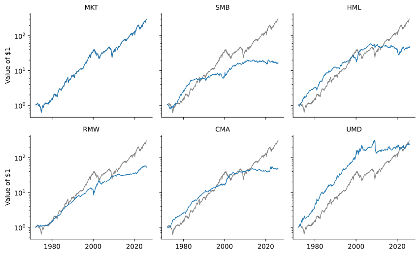
Table 2 reports the correlations among the six Fama-French factors. Most are small, which is part of what makes the factors useful: each captures a different source of comovement. The exception is HML and CMA, with a correlation of 0.68. Value firms tend to be firms that invest conservatively.
| MKT | SMB | HML | RMW | CMA | UMD | |
|---|---|---|---|---|---|---|
| MKT | 1.00 | 0.25 | -0.21 | -0.21 | -0.35 | -0.19 |
| SMB | 0.25 | 1.00 | 0.03 | -0.37 | -0.03 | -0.10 |
| HML | -0.21 | 0.03 | 1.00 | 0.14 | 0.68 | -0.20 |
| RMW | -0.21 | -0.37 | 0.14 | 1.00 | 0.08 | 0.07 |
| CMA | -0.35 | -0.03 | 0.68 | 0.08 | 1.00 | 0.01 |
| UMD | -0.19 | -0.10 | -0.20 | 0.07 | 0.01 | 1.00 |
Since Fama and French (2015) warned that the redundancy of HML might be specific to their sample, we can check it on the years since. Regressing HML on the other four factors from July 1963 to December 2013 gives an alpha of -0.1% a year, even though HML itself averaged 4.6%. From January 2014 to September 2026, HML averaged -0.8% a year, and its alpha relative to the other four factors is 0.5% (t = 0.18). The value premium disappeared after 2013, but the five-factor model accounts for that too: HML’s exposures to the other factors predicted its returns in both periods.
How Well Do the Models Price Assets?
Testing a Model with GRS
A model is tested on a set of assets by running (1) for each asset and asking whether all the alphas are jointly zero. The standard test is the F-statistic of Gibbons et al. (1989), the GRS test. It has a useful interpretation in terms of Sharpe ratios. If the alphas are zero, the factors span the tangency portfolio, and adding the test assets cannot raise the maximum Sharpe ratio. The GRS statistic grows with \frac{1 + \theta_{*}^{2}}{1 + \theta_{F}^{2}}, \tag{6} where \theta_{F} is the maximum Sharpe ratio attainable with the factors alone and \theta_{*} is the maximum Sharpe ratio attainable with the factors and the test assets together, both measured in the sample. A large statistic means that the test assets offer opportunities the factors do not span.
The 25 Size and Book-to-Market Portfolios
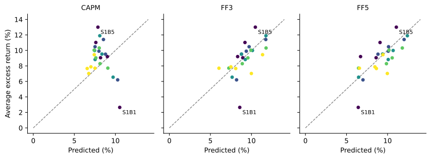
The classic test assets are the 25 portfolios formed on size and book-to-market that Fama and French (1993) introduced. Figure 2 plots their average excess returns against the returns three of the models predict, and Table 3 summarizes all six models.
| Mean absolute alpha (%) | Largest absolute t | GRS | p-value | |
|---|---|---|---|---|
| CAPM | 2.17 | 3.41 | 3.68 | < 0.001 |
| FF3 | 1.15 | 4.83 | 3.30 | < 0.001 |
| Carhart | 1.05 | 4.34 | 2.99 | < 0.001 |
| FF5 | 1.10 | 3.75 | 2.92 | < 0.001 |
| FF6 | 1.02 | 3.30 | 2.70 | < 0.001 |
| q-factor | 1.15 | 3.45 | 3.00 | < 0.001 |
Under the CAPM the predicted returns barely vary while the realized returns range from 2.6% to 13.0% a year. The multifactor models cut the average absolute alpha by more than half, from 2.2% to about 1.1%. Yet the GRS test rejects every model. With more than 50 years of data, even small alphas are statistically significant, and the small-growth portfolio, labeled S1B1, earns far less than any of the models predicts. A model can be rejected and still be useful; the question is whether its errors are small relative to the alternatives.
The Anomalies Revisited
Table 4 returns to the long-short decile spreads of the previous chapter and reports their alphas under each model. A bold entry has a t-statistic above 1.96 in absolute value.
| CAPM | FF3 | Carhart | FF5 | FF6 | q-factor | |
|---|---|---|---|---|---|---|
| Size | −0.14 | −0.74 | −0.79 | 0.08 | 0.03 | 1.01 |
| Value | 3.81 | −2.28 | −1.98 | −0.87 | −0.67 | 0.71 |
| Low beta | 6.36 | 4.31 | 1.33 | 0.30 | −1.88 | −1.62 |
| Momentum | 15.72 | 18.71 | 3.51 | 16.15 | 3.15 | 7.59 |
| Short-term reversal | −0.65 | −1.26 | 2.75 | 0.16 | 3.43 | 1.62 |
| Profitability | 6.54 | 5.89 | 5.34 | 0.04 | −0.01 | −0.03 |
| Investment | 5.69 | 2.84 | 1.64 | 0.21 | −0.36 | 0.17 |
| Accruals | 3.56 | 3.40 | 2.69 | 3.51 | 2.91 | 3.10 |
| Low volatility | 14.52 | 11.60 | 8.58 | 5.18 | 3.12 | 3.30 |
The CAPM leaves 6 of the nine spreads with significant alphas. Value is not among them in this sample, which reflects its weak returns since 2007. The three-factor model also leaves 6: it overcorrects for value, gives the low-beta spread a smaller alpha, and does nothing for profitability, investment, momentum, accruals or low volatility. The five-factor model leaves 3. It absorbs profitability, investment and low beta, as Fama and French (2016) found, and cuts the low-volatility alpha to 5.2% a year, but it leaves the momentum alpha as large as under the CAPM. Adding UMD brings the momentum alpha down to 3.2% a year in the six-factor model, which is still just significant. The q-factor model has no momentum factor, yet halves the momentum alpha, because its ROE factor has a correlation of 0.48 with UMD. Accruals keep a significant alpha in almost every model.
Comparing Models by Their Sharpe Ratios
The GRS interpretation in (6) suggests a way to rank models without choosing test assets. If a model’s factors span the tangency portfolio, no other asset can improve on their maximum Sharpe ratio. Since every factor is itself a portfolio that a competing model could use as a test asset, the better model is the one whose factors attain the higher maximum Sharpe ratio. Barillas and Shanken (2018) develop this idea into a Bayesian procedure for comparing all models built from a set of candidate factors, and find that models with momentum and with profitability and value factors updated monthly dominate the five-factor and q-factor models. Fama and French (2018) use the same metric to choose among versions of their own factors.
There is a direct link to the Treynor-Black model. Regress a new factor on the factors already in a model. If its alpha is \alpha_{k} and its residual volatility \sigma(e_{k}), adding it raises the maximum squared Sharpe ratio by the square of its information ratio: \theta_{\text{new}}^{2} = \theta_{\text{old}}^{2} + \left( \frac{\alpha_{k}}{\sigma(e_{k})} \right)^{2}. \tag{7} This is the Sharpe ratio result of the Treynor-Black model, with the existing factors in the role of the market and the new factor in the role of an active position. A factor with a high average return but zero alpha, like HML in the five-factor model, adds nothing.
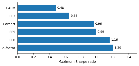
Figure 3 shows the maximum Sharpe ratio of each model’s factors over our sample. The market alone has a Sharpe ratio of 0.48. The six-factor model reaches 1.16, and the q-factor model 1.20. These numbers are in-sample: the weights that attain them are chosen with hindsight, so an investor could not have earned them. They are a fair comparison among models only because every model gets the same advantage.
The Factor Zoo
The search for anomalies has produced hundreds of candidate factors, which Cochrane (2011) called a “zoo”. Two questions follow: which of these factors are real, and how many does a model need?
On the first question the evidence is mixed. Hou et al. (2020) replicate 452 anomalies with NYSE breakpoints and value-weighted returns, which limits the influence of tiny stocks, and find that 65% cannot clear a t-statistic of 1.96, and that even replicated anomalies are much smaller than originally reported. Jensen et al. (2023) reach a more favorable conclusion with a Bayesian model of factor replication: most factors can be replicated, they cluster into 13 themes, and they work out of sample in a new data set covering 93 countries. Asness et al. (2013) find value and momentum premia in eight different markets and asset classes, with value and momentum negatively correlated with each other.
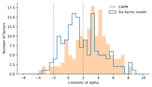
The factors of Jensen et al. (2023) are public, and the 153 U.S. factors cover our whole sample. Each buys the top third of stocks on one characteristic and sells the bottom third. Figure 4 compares the t-statistics of their alphas under the CAPM and the six-factor model. Under the CAPM, 72% of the factors have alphas significant at the 5% level. Under the six-factor model the share falls to 47%: six factors absorb much of the zoo, but far from all of it.
On the second question, recent work uses statistical methods designed for many factors at once, and finds that the information in hundreds of characteristics can be captured by a handful of well-chosen combinations, such as principal components, even if no short list of individual anomaly factors does the job. Estimation Risk and Shrinkage takes up these methods.
Using Factor Models
Factor models have three common uses in investment practice: they estimate the cost of equity, they provide risk models, and they serve as benchmarks for performance evaluation.
The Cost of Equity
A firm’s cost of equity is the expected return its shareholders require, and (2) delivers one: estimate the firm’s betas from the regression (1), estimate each factor premium by the factor’s average return, and add the risk-free rate. Firms mostly use the single beta of the CAPM. In the survey of Graham and Harvey (2001), 73.5% of chief financial officers always or almost always use the CAPM to estimate the cost of equity, while a multibeta model ranks third, behind average historical returns.
How precise are these estimates? Fama and French (1997) find that standard errors of more than 3% a year are typical for industry costs of equity, under both the CAPM and the three-factor model. Figure 5 repeats the exercise for Kenneth French’s 12 industry portfolios over January 1972 to December 2025. For each industry it shows the estimated risk premium \hat{\pmb{\beta}}_i'\hat{\pmb{\lambda}}, the betas times the average factor returns, with a band of two standard errors on each side. Both estimates carry sampling error, so \operatorname{V}\big(\hat{\pmb{\beta}}_i'\hat{\pmb{\lambda}}\big) \approx \pmb{\beta}_i' \operatorname{V}(\hat{\pmb{\lambda}})\, \pmb{\beta}_i + \pmb{\lambda}' \operatorname{V}(\hat{\pmb{\beta}}_i)\, \pmb{\lambda}. \tag{8}
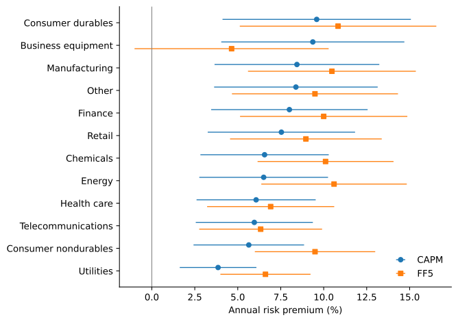
The standard errors range from 1.1 to 2.7% a year under the CAPM and from 1.3 to 2.9% under the five-factor model. Almost all of the uncertainty comes from the first term of (8). The betas are estimated precisely: their error alone contributes at most 0.7% a year. The factor premia are not. Even after 54 years of data, the average market excess return has a standard error of 2.1% a year, and every additional factor adds its own uncertainty. The betas are precise only as averages over the whole sample, though. Fama and French (1997) find that industry loadings vary strongly through time, so that for an industry’s current loadings, full-sample estimates are no more accurate than imprecise estimates from the latest three years of data. The standard errors in Figure 5 understate the uncertainty in a cost of equity for the years ahead.
The choice of model matters as much as the statistics. For business equipment, which loads negatively on HML, RMW and CMA because it is full of growth firms that invest heavily, the five-factor model cuts the risk premium from 9.4 to 4.6%. For chemicals and energy, which load positively on the same factors, it raises the risk premium by 3.5 and 4.1 percentage points. These gaps exceed a standard error of either estimate, so a multifactor cost of equity is not more precise than the CAPM’s. It is a different estimate.
Risk Models
The covariance matrix of many stocks follows from their loadings on a few factors, extending the logic of the index model. Rosenberg (1974) showed that there are significant common components of covariance beyond the market, and that the loadings on them are determined by observable characteristics of the firm, such as balance sheet data, industry membership and the past behavior of its returns. Commercial risk models descend from this work. Unlike the models of this chapter, they include industry factors alongside style factors such as size, value and momentum. Industries explain much of the comovement of stocks even though they carry no premium of their own, and a risk model must capture comovement whether or not it is priced.
Factor exposures are also a source of risk that no single fund controls. When many funds hold similar long-short positions, a forced sale by one moves the prices of the others. Khandani and Lo (2011) find that the losses of long-short equity strategies in August 2007 are consistent with such a market-wide deleveraging, together with a sudden withdrawal of market-making capital.
Benchmarks
A fund that earns high returns by tilting toward small value stocks or past winners has exposures an investor could buy cheaply, and only its alpha relative to the factors measures skill. Investors seem to apply a simpler standard. Using mutual fund flows to infer which model investors use, Berk and Binsbergen (2016) find that the CAPM comes closest, and Barber et al. (2016) find that investors attend mostly to market risk and treat returns from size, value, momentum and industry factors as alpha. The next chapter develops performance evaluation.
Practice Problems
These problems give you a chance to practice the concepts introduced in this chapter. Try to solve each one on your own before expanding the solution.
Problem 1 (An Expected Return from the Five-Factor Model) Hollis Grant estimates the cost of equity of Tamarack Industries (TMK). A five-factor regression gives loadings b = 1.1, s = 0.4, h = 0.3, r = 0.2 and c = -0.1. She uses factor premia of 7\% for MKT, 2\% for SMB, 3.5\% for HML, 3\% for RMW and 3\% for CMA, and a risk-free rate of 4\%. A CAPM regression gives TMK a beta of 1.15.
- Compute TMK’s expected return under the five-factor model.
- Compute its expected return under the CAPM.
- Which loadings explain the difference?
Solution
By (2), the expected excess return is 1.1 \times 7\% + 0.4 \times 2\% + 0.3 \times 3.5\% + 0.2 \times 3\% - 0.1 \times 3\% = 7.7\% + 0.8\% + 1.05\% + 0.6\% - 0.3\% = 9.85\%, so the expected return is 13.85\%.
4\% + 1.15 \times 7\% = 12.05\%.
The five-factor model adds 2.15\% for TMK’s tilts toward small, value and profitable firms, partly offset by its negative loading on CMA, which means it behaves like a firm that invests aggressively. The CAPM beta is higher than b because the single-factor regression attributes some of the SMB comovement to the market, but this adds only 0.35\%. The difference of 1.8\% is large for a cost of capital.
Problem 2 (Reading a Three-Factor Regression) A regression of the monthly excess returns of the Ashgrove Small Cap Fund on the three Fama-French factors gives \alpha = 0.15\% (t = 1.1), b = 0.95, s = 0.65, h = 0.45 and R^{2} = 0.93. A CAPM regression of the same returns gives \alpha = 0.40\% (t = 2.6) and \beta = 0.95. Over the sample, SMB averaged 0.18\% a month and HML 0.29\%.
- Describe the fund’s investment style from its loadings.
- Compute the part of the fund’s average return that comes from its SMB and HML exposures. Compare it with the difference between the two alphas.
- Has the fund manager shown skill? What would you tell an investor in the fund?
Solution
A market loading near one, a large positive SMB loading and a positive HML loading describe a fund that holds small value stocks.
The exposures contribute 0.65 \times 0.18\% + 0.45 \times 0.29\% = 0.117\% + 0.131\% = 0.248\% a month, which matches the difference of 0.40\% - 0.15\% = 0.25\% between the two alphas. Since the market loading is the same in both regressions, the CAPM alpha is the three-factor alpha plus the premia earned by the size and value tilts.
The three-factor alpha is not significant, so there is no evidence of skill beyond the tilts. Most of the fund’s CAPM alpha comes from holding small value stocks, which an investor can do more cheaply with a small-cap value index fund.
Problem 3 (Building SMB and HML) In one month, the six value-weighted portfolios formed on size (small S, big B) and book-to-market (low L, medium M, high H) return:
| Portfolio | S/L | S/M | S/H | B/L | B/M | B/H |
|---|---|---|---|---|---|---|
| Return (%) | 2.0 | 1.5 | 3.0 | 1.0 | 0.8 | 1.6 |
- Compute SMB and HML for the month.
- Why does HML average the small and big portfolios instead of using only big stocks?
Solution
SMB = (2.0 + 1.5 + 3.0)/3 - (1.0 + 0.8 + 1.6)/3 = 2.167\% - 1.133\% = 1.03\% and HML = (3.0 + 1.6)/2 - (2.0 + 1.0)/2 = 2.3\% - 1.5\% = 0.8\%.
Averaging over small and big makes HML hold the same weight in small stocks on its long and short sides, so it is roughly neutral to size and isolates the value effect. It also includes small stocks, where the value effect is strongest, without letting them dominate.
Problem 4 (Does a New Factor Add Anything?) The factors of a model have a maximum Sharpe ratio of 0.95 a year. A researcher proposes two new factors. Regressed on the model’s factors, factor A has an alpha of 2.4\% a year with a residual volatility of 8\%, and factor B has an alpha of zero, even though its average return is 4\% a year.
- What is the maximum Sharpe ratio after adding factor A?
- What is it after adding factor B? Why can a factor with a 4\% average return add nothing?
- With 50 years of data, what is the t-statistic of factor A’s alpha?
Solution
The information ratio of A is 2.4/8 = 0.3, so by (7) the new maximum Sharpe ratio is \sqrt{0.95^{2} + 0.3^{2}} = \sqrt{0.9025 + 0.09} = 0.996.
It stays at 0.95. Factor B’s average return is fully explained by its exposures to the existing factors, so any position in B can be replicated with those factors. This is the situation of HML in the five-factor model.
The t-statistic of an alpha is approximately its annual information ratio times the square root of the number of years, 0.3 \times \sqrt{50} = 2.12, barely significant even with half a century of data.
Problem 5 (The Valuation Identity) Three firms have book equity of $100 and market value of $150. Each is expected to earn the same equity earnings Y and make the same investment dB every year forever, so that (4) becomes M = (Y - dB)/r. Firm 1 has Y = 15 and dB = 6. Firm 2 has Y = 18 and dB = 6. Firm 3 has Y = 15 and dB = 9.
- Compute the expected return r of each firm.
- Which of the three predictions of the valuation identity does each comparison illustrate?
Solution
Solving r = (Y - dB)/M gives r_{1} = 9/150 = 6\%, r_{2} = 12/150 = 8\% and r_{3} = 6/150 = 4\%.
Firms 1 and 2 have the same book-to-market ratio and investment, but firm 2 is more profitable, so it has a higher expected return: the profitability prediction. Firms 1 and 3 have the same book-to-market ratio and profitability, but firm 3 invests more, so it has a lower expected return: the investment prediction. The book-to-market prediction compares firms with the same expected earnings and investment but different market values: a firm like firm 1 priced at $100 instead of $150 would have r = 9/100 = 9\%.
Problem 6 (A Fund That Rides Momentum) A fund has a three-factor alpha of 2.4\% a year. Adding UMD to the regression leaves the other loadings unchanged and gives a UMD loading of 0.30. UMD averaged 7\% a year over the sample.
- What is the fund’s four-factor alpha?
- What does the result say about the fund’s strategy and about the persistence of its returns?
Solution
2.4\% - 0.30 \times 7\% = 0.3\% a year.
Almost all of the three-factor alpha comes from holding past winners. A fund that tilts toward momentum stocks will tend to keep doing well while momentum pays, which looks like persistent skill. Carhart (1997) found that this is what drives the “hot hands” of mutual funds with high past returns.