The Term Structure in the Data
Forward Rates split every forward rate into the short rate that investors expect and a term premium, and showed that the term premium is the expected excess return of a long-term bond over a short one. The expectations hypothesis says the term premium is zero. This chapter takes the hypothesis to the data. It measures how much long-term Treasury bonds have earned over short-term ones, asks whether forward rates forecast future short rates or future bond returns, and looks at how the term premium and the risk of bonds have changed over time.
The data are the zero-coupon Treasury yields of Fama and Bliss (1987), for maturities of one to five years, from 1964 to 2025, and the Treasury yield curve of Bond Pricing for longer maturities. All yields and returns are continuously compounded, and an n-year bond held for a year becomes an (n - 1)-year bond, so its one-year excess log return is \mathit{rx}_{t+1}(n) = p_{t+1}(n - 1) - p_{t}(n) - y_{t}(1), where p is the log price.
Average Bond Returns
Table 1 reports the one-year excess returns of zero-coupon bonds with maturities of two to five years, from January 1964 to December 2024. Longer bonds earned more on average, 0.36% a year at two years and 1.04% at five, but they were also much more volatile, so their Sharpe ratios are modest. A 10-year zero, from the Treasury curve, earned 2.7% a year over Treasury bills from 1971 to 2025, with a volatility of 10.9% and a Sharpe ratio of 0.25, about half the 0.48 of the stock market over the same period. Long-term bonds have earned a premium, but a small one per unit of risk.
| Mean (%) | Volatility (%) | Sharpe ratio | |
|---|---|---|---|
| 2 years | 0.36 | 1.70 | 0.21 |
| 3 years | 0.68 | 3.12 | 0.22 |
| 4 years | 0.97 | 4.34 | 0.22 |
| 5 years | 1.04 | 5.38 | 0.19 |
Average returns are a weak test of the expectations hypothesis. Over 1964 to 2025, interest rates first rose and then fell for four decades, which raised the realized returns of long-term bonds after 1981 whatever their expected returns were. The sharper tests ask whether the forward rates of each date forecast what happened next.
Do Forward Rates Forecast Short Rates?
Under the expectations hypothesis, the forward rate for the year from n - 1 to n is the market’s forecast of the one-year rate in n - 1 years. Fama and Bliss (1987) tested this by regressing the change in the one-year yield over the next n - 1 years on the forward spread, the gap between the forward rate and today’s one-year yield: y_{t+n-1}(1) - y_{t}(1) = a + b \left( f_{t}(n - 1, n) - y_{t}(1) \right) + \varepsilon_{t+n-1}. \tag{1} If forward rates are the expected future rates, the slope b is one. The same forward spread can be used to forecast the excess return of the n-year bond over the next year, \mathit{rx}_{t+1}(n) = a + b \left( f_{t}(n - 1, n) - y_{t}(1) \right) + \varepsilon_{t+1}, \tag{2} and under the hypothesis this slope is zero, since a bond’s expected excess return is a constant term premium. The two regressions are two sides of the same coin. For n = 2, the identity for the excess return of the 2-year bond in Forward Rates gives f_{t}(1, 2) - y_{t}(1) = \left( y_{t+1}(1) - y_{t}(1) \right) + \mathit{rx}_{t+1}(2), so the two slopes add up to exactly one: whatever the forward spread does not forecast about the future short rate, it forecasts about the bond’s return.
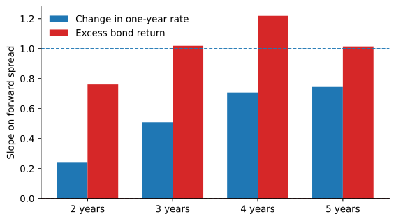
Figure 1 shows the slopes, and Table 2 the details. Forward rates do contain information about future short rates, and more so at longer horizons: the slope rises from 0.24 for the change over one year to 0.74 over four years, as Fama and Bliss (1987) found. But over the next year, most of the forward spread forecasts the bond’s excess return, with slopes of 0.8 to 1.2 and t-statistics above 3.1. When the forward rate is high relative to today’s yield, long-term bonds tend to earn more than short ones over the following year, which is what a time-varying term premium means.
| Slope | t-stat. | R-squared | Slope | t-stat. | R-squared | |
|---|---|---|---|---|---|---|
| 2 years | 0.24 | 1.18 | 0.01 | 0.76 | 3.77 | 0.10 |
| 3 years | 0.51 | 1.76 | 0.05 | 1.02 | 4.02 | 0.11 |
| 4 years | 0.71 | 2.96 | 0.10 | 1.22 | 4.07 | 0.13 |
| 5 years | 0.74 | 3.43 | 0.12 | 1.01 | 3.06 | 0.07 |
Campbell and Shiller (1991) ran a test in the other direction. Under the expectations hypothesis, a steep yield curve means that short rates are expected to rise, and to keep the expected return of a long bond equal to that of a short one, the long yield must rise over the next year as well, with a slope of one in a regression of the change in the long yield on (y_{t}(n) - y_{t}(1))/(n - 1). They found the opposite, and so do our data: the slopes are negative, from -0.52 at two years to -1.23 at five. A steep curve is followed, on average, by falling long yields, which raises the returns of long bonds. In their words, a high yield spread forecasts rising short rates over the long term but a declining long yield over the short term.
A Single Factor in Bond Risk Premia
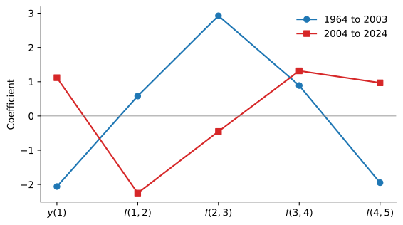
Cochrane and Piazzesi (2005) went further. Instead of one forward rate at a time, they regressed the average excess return of the two- to five-year bonds on all five forward rates at once, the one-year yield and the four forwards. A single combination of forward rates, with a tent shape, forecast the excess returns of all the bonds, with an R^{2} of up to 0.44 in their sample from 1964 to 2003. Figure 2 shows the coefficients in our data. From 1964 to 2003 the tent is clear and the R^{2} is 0.35, close to theirs. From 2004 to 2024 the coefficients look different, and the R^{2} is 0.21.
How much to trust such regressions is debated. The forecasting variables are persistent and the returns overlap, and Bauer and Hamilton (2018) show that the usual tests then overstate the evidence that variables beyond the level, slope and curvature of the yield curve forecast bond returns. The broad conclusion survives: forward rates forecast bond returns better than they forecast short rates, so term premia vary over time. Dai and Singleton (2002) show that term structure models in which the price of interest rate risk changes with the state of the economy reproduce both the Fama-Bliss and the Campbell-Shiller findings.
Term Premia over Time
If term premia vary, how large are they now? A forward rate is observed, but the expected short rate is not, so the term premium has to be estimated with a model. The Federal Reserve Bank of New York publishes estimates from the model of Adrian et al. (2013), which forecasts short rates with the principal components of the yield curve. Figure 3 shows its estimate of the term premium in the 10-year yield, the part of the yield above the average short rate expected over ten years.
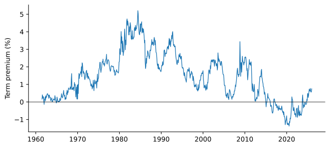
The estimated premium peaked at 5.2% in May 1984, when inflation had been high and volatile and investors feared it would return. It then declined for three decades, was negative in 52% of the months from 2011 to 2021, reached -1.4% in July 2020, and was 0.75% at the end of 2025. A negative term premium means that investors accepted a lower expected return on long-term bonds than on rolling short ones.
Several forces move the premium. The first is the supply of long-term bonds. Greenwood and Vayanos (2014) find that when the Treasury’s debt has a longer maturity relative to GDP, yields and subsequent excess returns of long-term bonds are higher, consistent with the preferred habitat view of Forward Rates: arbitrageurs must be paid to absorb the extra duration. The Federal Reserve’s purchases of long-term bonds after 2008 worked in the opposite direction. The second is the special value of Treasuries. Krishnamurthy and Vissing-Jorgensen (2012) estimate that the liquidity and safety of Treasuries lowered their yields by 73 basis points on average from 1926 to 2008, and that the effect is larger when Treasuries are scarce. The third is the risk of the bonds themselves.
Bonds as Hedges
A term premium is compensation for risk, and the risk that matters is how bonds do when other investments do badly. Figure 4 shows the correlation between the monthly excess returns of a 10-year zero and the stock market over rolling five-year windows. It was positive in the 1970s, 1980s and 1990s, 0.29 over 1971 to 1999, and negative in the 2000s and 2010s, -0.11 over 2000 to 2025 as a whole and close to -0.6 at its lowest. After the inflation of 2021 and 2022 it was mixed for a while, between -0.25 and 0.26 in 2022 and 2023, and it was clearly positive again in 2024 and 2025, up to 0.54.
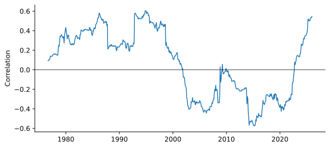
Campbell et al. (2017) explain the swings with inflation. When the main risk is inflation, as in the 1970s and early 1980s, bad news about inflation lowers both stock and bond prices, so bonds are risky and earn a high term premium. When the main risk is a recession with falling inflation, as in the downturns of 2001 and 2007 to 2009, bond prices rise when stock prices fall, so bonds hedge stock market risk and investors accept a low or negative term premium. The figure, the term premium estimates and their model all tell the same story: the term premium is high when bonds are inflation bets and low when they are deflation hedges.
What changes the mix of shocks? Campbell et al. (2020) estimate that the correlation between inflation and the output gap switched from negative to positive in 2001: before, high inflation came with weak output, as in a supply shock, and after, with strong output, as in a demand shock. Since higher inflation lowers bond returns and higher output raises stock returns, the switch turned the stock-bond correlation from positive to negative. Pflueger (2025) adds monetary policy. In her model, bonds and stocks move together only when supply shocks are volatile and the Federal Reserve responds strongly to inflation, as in the 1980s. After the pandemic, supply shocks returned, but bond-stock betas stayed negative through 2022, which she attributes to a monetary policy framework that was more inertial and less focused on inflation than in the 1980s, and that raised its response to inflation only late. The rolling correlation in Figure 4, which extends three years beyond her data, turned clearly positive only in 2024. What moved bond yields in this latest episode, though, was not expected inflation.
Real Rates since 2021
A nominal yield is the sum of a real yield, at which inflation-protected Treasuries (TIPS) trade, and breakeven inflation, the gap between the nominal and TIPS yields of the same maturity. Breakeven inflation measures expected inflation plus a premium for inflation risk, less a liquidity premium on TIPS. Long-run expected inflation barely moved after 2021: the 10-year breakeven averaged 2.33% in 2025, about where it was from 2003 to 2007, 2.35%, when the stock-bond correlation was strongly negative. Table 3 splits the monthly changes in the 10-year yield into these two parts and asks which one moves with stocks.
| Nominal yield | Breakeven | Real yield | Real yield share (%) | |
|---|---|---|---|---|
| 2010 to 2019 | 0.49 | 0.66 | 0.07 | 60 |
| 2021 to 2025 | -0.54 | 0.25 | -0.69 | 84 |
In the 2010s, the hedge worked through inflation expectations. When stocks fell, breakevens fell with them, nominal yields dropped and bonds rallied, while changes in real yields were unrelated to stock returns. Since 2021, the real yield has accounted for 84% of the variance of yield changes, and it rises when stocks fall. From December 2020 to December 2025, the 10-year real yield rose from -1.06% to 1.93%, while breakeven inflation moved only from 1.99% to 2.25%. A higher real rate raises the discount rate on every asset, so stocks and bonds fall together. Government debt is a claim on future taxes and stocks a claim on future profits, so when both lose value at once the shock is economy-wide. Neither asset hedges the other, and investors as a whole cannot get rid of the risk, so they must be paid to bear it, consistent with the rise of the term premium in Figure 3 after 2022. Molenaar et al. (2024), with data back to 1875, find that since 1951 the stock-bond correlation has been high when real short rates are high as well as when inflation is high, and that bond risk premiums rise with the correlation.
Why real rates now rise when stocks fall is an open question. One candidate is monetary policy: with inflation above target, the Federal Reserve cannot cut rates when stocks fall, and hawkish surprises raise real rates and lower stock prices, the mechanism of Pflueger (2025). Another is the real term premium: when investors doubt fiscal policy, the return they require to hold government debt rises. In the fiscal theory of the price level of Cochrane (2023), government debt is valued like a stock, so a higher discount rate on it lowers the value of bonds and, through the same discount rate, of stocks. A caution comes from Duffee (2023), who finds that from 1978 to 2016 neither the theories that emphasize inflation nor those that emphasize real rates match how macroeconomic news moves stock returns and bond yields.
For an investor, the evidence has three parts. Long-term Treasury bonds have earned a premium over bills, but a small one per unit of risk. The premium varies over time, and forward rates forecast part of that variation, although the forecasts are less reliable than their in-sample fit suggests. And the role of bonds in a portfolio depends on what moves yields in bad times. When bad news lowers expected inflation and short rates, falling yields make bonds a cushion; when real rates rise as stocks fall, as after 2021, the same bonds lose money alongside stocks.
Practice Problems
These problems give you a chance to practice the concepts introduced in this chapter. Try to solve each one on your own before expanding the solution.
Problem 1 (An Excess Bond Return) The prices of zero-coupon bonds with a face value of $1 are 0.9600 for one year, 0.9200 for two years and 0.8800 for three years. A year later, the price of a two-year zero is 0.9300.
- Compute the one-year yield and the log prices of the bonds, all continuously compounded.
- Compute the one-year excess log return of the three-year bond.
- Compute the forward rate f(2, 3) and the forward spread f(2, 3) - y(1).
Solution
y(1) = -\ln 0.96 = 4.08\%. The log prices are p(3) = \ln 0.88 = -0.1278 today and p(2) = \ln 0.93 = -0.0726 a year later.
\mathit{rx}(3) = -0.0726 - (-0.1278) - 0.0408 = 1.44\%.
f(2, 3) = p(2) - p(3) = \ln 0.92 - \ln 0.88 = 4.45\%, so the forward spread is 4.45\% - 4.08\% = 0.37\%. The bond’s excess return of 1.44% was well above the spread, because the two-year yield a year later, -\ln(0.93)/2 = 3.63\%, was lower than the forward rates implied.
Problem 2 (Two Slopes That Add Up to One) Use the identity f_{t}(1, 2) - y_{t}(1) = \left( y_{t+1}(1) - y_{t}(1) \right) + \mathit{rx}_{t+1}(2).
- Show that if both sides are regressed on the forward spread f_{t}(1, 2) - y_{t}(1), the slopes of the regressions of the change in the one-year yield and of the excess return add up to one.
- In a sample, the slope for the change in the one-year yield is 0.3. What is the slope for the excess return? What does each extreme, 1 and 0, say about the term premium?
Solution
The OLS slope of a sum of two variables on a regressor is the sum of their slopes. Regressing the forward spread on itself gives a slope of one, so the two slopes add up to one.
0.7. A slope of one for the rate change, and zero for the return, is the expectations hypothesis: the forward spread forecasts only the future short rate, and the term premium is constant. A slope of zero for the rate change, and one for the return, means the forward spread forecasts only the term premium, so a high forward rate signals a high expected return and nothing about future short rates.
Solution
The yield is the expected average short rate plus the term premium, so the expected average short rate is 4.26\% - 0.75\% = 3.51\%.
0.9\% + 1.2\% = 2.1\%. Investors accept a negative term premium when long-term bonds are a hedge: if bond prices tend to rise when stocks and the economy do badly, as in 2001 and 2008, holding them lowers the risk of a portfolio, and investors pay for that protection with a lower expected return. Purchases of long-term bonds by the Federal Reserve and the safety value of Treasuries also pushed the premium down.
Problem 4 (Bonds in a Portfolio) A portfolio holds 60% in stocks, with a volatility of 16%, and 40% in long-term bonds, with a volatility of 11%.
- Compute the portfolio’s volatility when the correlation between stocks and bonds is -0.3, as in the 2010s, and when it is +0.5, as in the early 1980s and again after 2022.
- How does the change in correlation relate to the term premium that investors require on bonds?
Solution
The variance is 0.6^{2} \times 0.16^{2} + 0.4^{2} \times 0.11^{2} + 2 \times 0.6 \times 0.4 \times \rho \times 0.16 \times 0.11. With \rho = -0.3 it is 0.009216 + 0.001936 - 0.002534 = 0.008618, a volatility of 9.3%. With \rho = +0.5 it is 0.009216 + 0.001936 + 0.004224 = 0.015376, a volatility of 12.4%.
When bonds are negatively correlated with stocks, they lower the risk of a typical portfolio, and investors are willing to hold them at a low or negative term premium. When the correlation is positive, bonds add to the risk of the portfolio, and investors require a higher premium to hold them.
Problem 5 (Real Yields and Breakeven Inflation) At the end of 2020, the 10-year nominal Treasury yield was 0.93% and the 10-year TIPS yield was -1.06\%. At the end of 2025, they were 4.18% and 1.93%.
- Compute the 10-year breakeven inflation rate at both dates.
- How much of the rise in the nominal yield came from the real yield, and how much from breakeven inflation?
- Why does a rise in real yields tend to lower stock prices as well as bond prices, while a rise in breakeven inflation that comes with good news about growth need not?
Solution
Breakeven inflation is the nominal yield minus the TIPS yield: 0.93\% - (-1.06\%) = 1.99\% at the end of 2020 and 4.18\% - 1.93\% = 2.25\% at the end of 2025.
The nominal yield rose by 3.25 percentage points. The real yield rose by 1.93\% - (-1.06\%) = 2.99 points and breakeven inflation by 2.25\% - 1.99\% = 0.26 points, so about 92% of the rise came from the real yield.
The real yield is part of the discount rate for every cash flow, so a higher real rate lowers the present value of both bond payments and dividends. Higher breakeven inflation that comes with stronger growth also brings higher expected dividends, which can raise stock prices even as bond prices fall, the pattern of the 2010s.