The Greeks
The Greeks measure how the value of an option portfolio responds to changes in its inputs: the underlying asset price, time, volatility, and the risk-free rate. Traders use them both to understand risk exposure and to construct hedges. Delta captures first-order price sensitivity; gamma captures the curvature of that sensitivity; theta captures the erosion of value with time; vega captures exposure to changes in volatility; and rho captures exposure to interest rate moves. Together, they give a complete local picture of an option portfolio’s risk.
From Replication to Hedging
The Black-Scholes model prices an option by replication: holding N_{S} = \partial V / \partial S shares and rebalancing continuously reproduces the option exactly. A trading desk that sells an option can hold the same portfolio as a hedge. Sometimes a static hedge with other options is available, but often it is not feasible or too expensive, and the desk hedges dynamically. A position hedged this way is delta neutral.
In practice the desk cannot rebalance continuously. It trades at discrete times, say once a day or once a week, and between trades the hedge is imperfect. The other Greeks measure what goes wrong between trades and what the position is exposed to besides the stock price.
Delta
The delta of an option (or portfolio) measures its sensitivity to the underlying asset price. Formally, if we denote by V the value of a portfolio (possibly containing the stock, risk-free bonds and/or options), the delta of the portfolio is defined as: \Delta = \frac{\partial V}{\partial S} The delta of a portfolio is the sum of the deltas of its positions. A share of the stock has a delta of one and a bond has a delta of zero, so the desk adjusts the delta of a portfolio by trading the stock. The delta of a European call or put is the hedge ratio of The Black-Scholes Model.
Example 1 Consider a non-dividend paying stock that currently trades at $50. The money-market risk-free rate is 5% per year with continuous compounding, and the volatility of log-returns is 25% per year. Compute the delta of a European call option with maturity 6 months and strike of $50. d_{1} = \frac{\ln(50/50) + (0.05 + \frac{1}{2}(0.25)^{2})(0.5)}{0.25\sqrt{0.5}} = 0.2298
The delta is then equal to \operatorname{Φ}(d_{1}) = 0.591.
The next example follows a desk that hedges this call once a week.
Example 2 Consider a non-dividend paying stock that currently trades at $50. A trader just sold 50 call option contracts (5,000 options) written on the stock. The current option price is $4.13 and the option’s delta is 0.591. The money-market risk-free rate is 5% per year with simple compounding.
- First hedge: The delta of the position is -5{,}000 \times 0.591 = -2{,}955. To delta hedge the position, the trader buys 2,955 shares for a cost of $147,750. By writing the calls, the trader receives 5{,}000 \times 4.13 = \$20{,}650, which amounts to a net expense of $127,100 that the trader borrows. The trader borrows at the risk-free rate.
- Price Change: During the next week, the stock price increases to $50.53, the option price increases to $4.35, and the delta changes to 0.612. The delta of the option position changes to -5{,}000 \times 0.612 = -3{,}060.
- Profit & Loss: The long stock position is now worth 2{,}955 \times 50.53 = \$149{,}316.15, whereas the short call position is worth -5{,}000 \times 4.35 = -\$21{,}750. The loan now accrues to -127{,}100 \left(1 + \frac{0.05}{52}\right) = -\$127{,}222.21. The weekly P&L is then 149{,}316.15 - 21{,}750 - 127{,}222.21 = \$343.94, which is a small percentage of the total exposure.
- Hedge re-balancing: The trader buys an additional 3{,}060 - 2{,}955 = 105 shares to maintain delta neutrality. The cost of the additional shares is 105 \times 50.53 = \$5{,}305.65, which the trader borrows. The total loan is now 127{,}222.21 + 5{,}305.65 = \$132{,}527.86.
To maintain delta neutrality, we must continue the same process week after week until the expiration of the options.
A perfect hedge would earn nothing, so the $343.94 is a hedging error. We explain where it comes from in The Profit of a Delta Hedge, once we have gamma and theta.
Example 3 Consider:
- A long position in 100,000 call options (1,000 contracts) with strike price $100 and expiration in 9 months. The delta of each option is 0.597.
- A short position in 200,000 call options (2,000 contracts) with strike $110 and expiration in 6 months. The delta of each option is 0.368.
- A short position in 50,000 put options (500 contracts) with strike $90 and expiration in 3 months. The delta of each option is -0.162.
The delta of the portfolio is: 100{,}000 \times 0.597 - 200{,}000 \times 0.368 - 50{,}000 \times (-0.162) = -5{,}800
The portfolio can then be made delta neutral by buying 5,800 shares.
Gamma
The gamma (\Gamma) of a portfolio measures the rate of change of the portfolio’s delta with respect to the price of the underlying asset, i.e. \Gamma = \frac{\partial \Delta}{\partial S} = \frac{\partial^{2} V}{\partial S^{2}}
Gamma is the reason a delta hedge must be rebalanced. When gamma is small, delta changes slowly and the portfolio is kept delta neutral without many changes. On the other hand, when gamma is high, it is important to monitor the portfolio frequently and adjust delta neutrality as needed.
The gamma for European call and put options is: \Gamma_{C} = \Gamma_{P} = \frac{e^{-\delta T} \mathop{\Phi^{'}}(d_{1})}{S \sigma \sqrt{T}} = \frac{K e^{-r T} \mathop{\Phi^{'}}(d_{2})}{S^{2} \sigma \sqrt{T}}
Example 4 Let’s compute the gamma of the option in Example 1. Using d_{1} = 0.2298 from that example, we compute \mathop{\Phi^{'}}(d_{1}) = \frac{1}{\sqrt{2 \pi}} e^{-\frac{1}{2} (0.2298)^{2}} = 0.3885. The gamma of the option is then: \Gamma = \frac{\mathop{\Phi^{'}}(d_{1})}{S \sigma \sqrt{T}} = \frac{0.3885}{50 (0.25) \sqrt{0.5}} = 0.0440
Gamma and Delta Neutrality
According to Itô’s lemma, the change in the value of a portfolio is dV = \frac{\partial V}{\partial S} dS + \frac{1}{2} \frac{\partial^{2} V}{\partial S^{2}} (dS)^{2} + \frac{\partial V}{\partial t} dt = \Delta dS + \frac{1}{2} \Gamma (dS)^{2} + \frac{\partial V}{\partial t} dt In a delta-neutral portfolio the first term vanishes, and over a short interval \Delta V \approx \frac{1}{2} \Gamma (\Delta S)^{2} + \frac{\partial V}{\partial t} \Delta t A delta-neutral portfolio is therefore not riskless. Its value moves with the square of the stock price change, and the sign of gamma decides whether large moves help or hurt.
Figure 1 shows both terms for the call of Example 1. The left panel plots the call against the stock price together with the value of \Delta = 0.591 shares and the cash that replicate it, a line tangent to the call at $50. The call lies above the line on both sides, and the gap, the value of a long call hedged with a short position in those shares, grows with the square of the move. The right panel adds the passage of time. Over one week the call also loses time value, so the hedged position gains only if the stock ends the week below $48.33 or above $51.79, and loses in between. In the week of Example 2 the stock rose to $50.53, inside that range, so the desk, which was short the calls, made money.
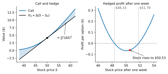
Example 5 Suppose that the gamma of a delta-neutral portfolio is 10,000. A jump of +$2 or -$2 in the underlying asset will approximately increase the value of the portfolio by \frac{1}{2} 10{,}000 \times 2^{2} = \$20{,}000.
The stock and the bond have zero gamma, so the gamma of a portfolio can only be changed by trading options.
Example 6 A trader’s portfolio is delta-neutral and has a gamma of 5,000. The delta and gamma of a traded call option are 0.52 and 1.60, respectively. The trader wants to make the portfolio both delta and gamma-neutral.
The portfolio can be made gamma-neutral by selling \frac{5{,}000}{1.60} = 3{,}125 call options. The portfolio can now be made delta-neutral by buying 0.52 \times 3{,}125 = 1{,}625 shares of the underlying asset. Note that the shares have zero gamma, so they do not change the gamma of the portfolio but only affect its delta.
Theta
The theta (\Theta) of a portfolio (V) captures the rate of change in value of that portfolio with respect to the passage of time, i.e. \Theta = \frac{\partial V}{\partial t}
The theta is also referred to as the time-decay of the portfolio. For European call and put options we have that: \begin{aligned} \Theta_{C} & = - e^{-\delta T} \frac{S \mathop{\Phi^{'}}(d_{1}) \sigma}{2 \sqrt{T}} - r K e^{-r T} \operatorname{Φ}(d_{2}) + \delta S e^{-\delta T} \operatorname{Φ}(d_{1}) \\ \Theta_{P} & = - e^{-\delta T} \frac{S \mathop{\Phi^{'}}(d_{1}) \sigma}{2 \sqrt{T}} + r K e^{-r T} \operatorname{Φ}(-d_{2}) - \delta S e^{-\delta T} \operatorname{Φ}(-d_{1}) \end{aligned}
Theta and Gamma
The Black-Scholes differential equation ties theta to the other Greeks: (r - \delta) S \frac{\partial V}{\partial S} + \frac{1}{2} \sigma^{2} S^{2} \frac{\partial^{2} V}{\partial S^{2}} + \frac{\partial V}{\partial t} = r V which can be re-written using the Greeks as: (r - \delta) S \Delta + \frac{1}{2} \sigma^{2} S^{2} \Gamma + \Theta = r V
Hence, for a delta-neutral portfolio we have that: \frac{1}{2} \sigma^{2} S^{2} \Gamma + \Theta = r V
Therefore, when theta is large and positive, the gamma of a portfolio tends to be large and negative, and vice-versa. This is why traders monitor theta closely: in a delta-neutral book, theta is the price paid, or earned, for gamma.
The Profit of a Delta Hedge
Consider a desk that is long an option and short N_S = \Delta shares, with the difference V - N_S S financed at the risk-free rate. We write the number of shares as N_S, as in the replicating portfolio of the binomial model, because in this section \Delta also marks changes over the interval, and \Delta S is the change in the stock price, not delta times S. Over a short interval \Delta t the desk gains \Delta V - N_S (\Delta S + \delta S \Delta t) on the option and the shares, including the dividends it pays on the short shares, and pays r (V - N_S S) \Delta t in interest. Replacing \Delta V by its Itô approximation and \Theta by its value from the Black-Scholes equation, the profit of the hedged position is \frac{1}{2} \Gamma (\Delta S)^{2} + \Theta \Delta t - r (V - N_S S) \Delta t - \delta N_S S \Delta t =\frac{1}{2} \Gamma S^{2} \left[ \left(\frac{\Delta S}{S}\right)^{2} - \sigma^{2} \Delta t \right]. The term in brackets compares the squared return the stock actually delivered with the variance \sigma^{2} \Delta t used to price the option. A long-gamma position gains when the stock moves more than the volatility implies and loses its theta when the stock moves less. A short-gamma position, like the desk that sold calls, earns theta in quiet markets and loses when the stock moves a lot.
Example 7 In Example 2 the desk is short 5,000 calls with S = 50, \sigma = 0.25, and, from Example 4, \Gamma = 0.0440 per option. Over one week the stock rose from $50 to $50.53, a return of 0.53/50 = 1.06\%. Then \left(\frac{\Delta S}{S}\right)^{2} = 0.000112 \quad \text{and} \quad \sigma^{2} \Delta t = \frac{0.25^{2}}{52} = 0.001202. The stock moved less than its volatility implies, so the short calls gain about 5{,}000 \times \frac{1}{2} (0.0440) (50)^{2} \times (0.001202 - 0.000112) = \$299.75, which accounts for most of the $343.94 profit of the week. The rest comes from applying an instantaneous formula to a whole week, over which gamma and theta themselves change.
The example follows a single week. Figure 2 follows the desk’s hedge over the whole life of the option. It simulates 500 stock paths, each with its own volatility between 10% and 40%, and on each path the desk sells the call of Example 1 at the Black-Scholes price with \sigma = 25\% and delta hedges it once a week until maturity. The profit is almost a function of a single number, the volatility the path actually delivered. Paths that turned out calmer than 25% make money and paths that turned out more volatile lose it, close to the line C(25\%) - C(\sigma_{\mathit{realized}}), the profit the desk would lock in if it had known the realized volatility in advance and hedged with it. The scatter around the line comes from weekly rebalancing and from when the large moves happen, since they cost more when gamma is high.
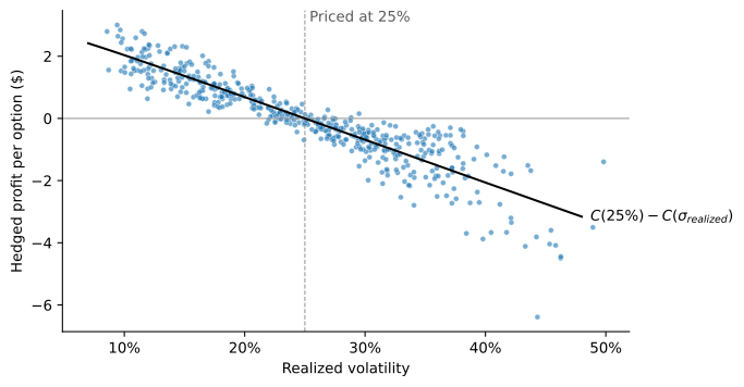
Trading desks run the calculation of Example 7 every day. A P&L attribution report, often called the P&L explain, splits the day’s profit into a delta part, a gamma part, a theta part, a vega part, and an unexplained residual, as the example did for one week. A large residual tells risk managers that the Greeks no longer describe the book.
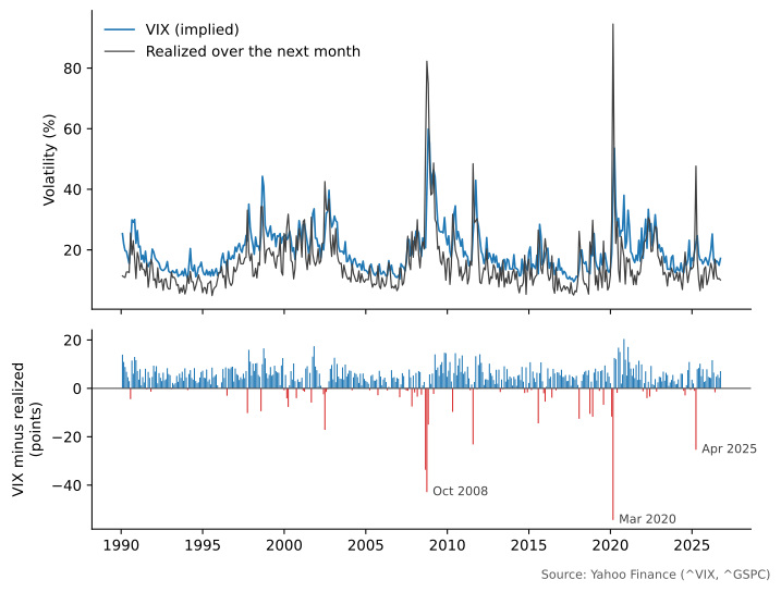
The formula also says what to expect on average. If the \sigma in option prices matched, on average, the volatility the stock then delivers, delta-hedged options would earn nothing. Bakshi and Kapadia (2003) find instead that delta-hedged long calls on the S&P 500 lost money from 1988 to 1995, about 8% of the option value for at-the-money calls. They attribute the losses to a negative volatility risk premium: market volatility tends to rise when the market falls, so options are hedges against market declines, and investors pay a premium to hold them. A desk that sells options and delta hedges collects that premium on average, as compensation for the large losses it takes when the market crashes.
Figure 3 shows the same premium over a longer period with the VIX, the implied volatility of 30-day S&P 500 index options computed by Cboe. Each month it compares the VIX at the end of the month with the volatility the index delivered over the following month. From 1990 to September 2026, the VIX was higher in 84% of months, by 4.1 points on average. The exceptions are the crashes, when realized volatility overshot the VIX by tens of points: October 2008, March 2020, and April 2025.
Transaction Costs
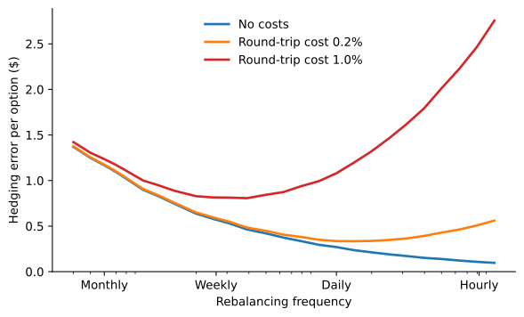
The profit formula ignores the cost of trading. Rebalancing more often shrinks the gamma error, but every trade costs money, and a hedge rebalanced continuously would trade without limit. Leland (1985) shows that with Black-Scholes deltas, the hedging error after transaction costs does not shrink as rebalancing becomes more frequent. He proposes instead to hedge with the Black-Scholes formula evaluated at a modified variance, \hat{\sigma}^{2} = \sigma^{2} \left(1 + \sqrt{\frac{2}{\pi}} \frac{k}{\sigma \sqrt{\Delta t}}\right), where k is the round-trip transaction cost as a fraction of the amount traded and \Delta t is the time between rebalancings. The higher volatility makes the option more expensive to replicate, and the difference with the Black-Scholes price is the cost of the hedge. A buyer who offsets the option by trading in the opposite direction uses a lower variance, so transaction costs turn the single Black-Scholes price into a band.
Figure 4 shows the trade-off for a short position in the call of Example 1, on simulated paths whose volatility is the 25% used to price and hedge it, so that rebalancing and its costs are the only sources of error. Without costs, the hedging error falls with the square root of the number of trades: rebalancing four times as often halves it. With costs, the amount paid grows with the number of trades, and beyond some frequency hedging more often makes the hedge worse. The best frequency falls as costs rise, from about daily with a round-trip cost of 0.2% to about weekly with 1%.
Buehler et al. (2019), researchers at J.P. Morgan and ETH Zürich, solve the problem numerically. In deep hedging, a neural network learns the hedging strategy from simulated market paths, choosing its trades to minimize a risk measure of the hedged profit after transaction costs and trading limits, and it can hedge with liquid options as well as with the stock. Without transaction costs, the learned strategy recovers the model hedge; with costs, it trades off hedging error against the cost of trading, a choice the Greeks alone cannot make. Risk limits and P&L reports are still expressed in Greeks, so learned hedges complement them rather than replace them.
The profit of a delta hedge depends on how volatile the stock turns out to be relative to the \sigma in the price. Uncertainty about that volatility is the risk that vega measures.
Vega
We met vega in The Black-Scholes Model as the sensitivity of the option price to volatility. In practice it is computed with respect to the implied volatility, since that is the volatility traders quote: \mathcal{V} = \frac{\partial V}{\partial \sigma}
The vega for European call and put options is: \mathcal{V}_{C} = \mathcal{V}_{P} = S e^{-\delta T} \mathop{\Phi^{'}}(d_{1}) \sqrt{T} = K e^{-r T} \mathop{\Phi^{'}}(d_{2}) \sqrt{T}
Usually vega risk is more relevant for longer maturity options, whereas gamma risk is more prominent for shorter maturity options. As with gamma, the stock and the bond have zero vega, so vega can only be hedged with other options, and hedging gamma and vega at the same time takes two different options.
Example 8 Consider a portfolio that is delta neutral, with a gamma of -5,000 and a vega of -8,000. The options shown in the table below can be traded.
| Delta | Gamma | Vega | |
|---|---|---|---|
| Original Portfolio | 0 | -5,000 | -8,000 |
| Option 1 | 0.6 | 0.5 | 2.0 |
| Option 2 | 0.5 | 0.8 | 1.2 |
The portfolio can be made vega neutral by including a long position in 4,000 units of Option 1. This would increase delta to 2,400 and require that 2,400 units of the asset be sold to maintain delta neutrality. The gamma of the portfolio would change from -5,000 to -3,000.
To make the portfolio both gamma and vega neutral, both Option 1 and Option 2 can be used. We must then solve: \begin{aligned} -5{,}000 + 0.5 N_{1} + 0.8 N_{2} = 0 \\ -8{,}000 + 2.0 N_{1} + 1.2 N_{2} = 0 \end{aligned}
This yields N_{1} = 400 and N_{2} = 6{,}000. The new delta is 400 \times 0.6 + 6{,}000 \times 0.5 = 3{,}240. Hence, we sell 3,240 units of the underlying asset to maintain delta-neutrality.
Even a book that is delta, gamma, and vega neutral is not riskless. Dealers trade at discrete times, volatility changes in ways a single vega does not capture, and prices jump. Garleanu et al. (2009) argue that, because of this unhedgeable risk, option prices depend on demand: dealers who take the other side of what end users want to trade charge for the risk they cannot hedge. Using CBOE data from 1996 to 2001, they find that end users are net long S&P 500 index options, with large positions in out-of-the-money puts, so dealers are net short, and the dealers’ delta-hedged profits and losses swung by as much as $100 million a day. Demand pressure helps explain why index options are expensive and why their implied volatility falls so steeply with the strike, the skew of The Volatility Surface.
Dealers set these prices through the quotes they post, and increasingly an algorithm posts them. In the model of Baldacci et al. (2021), a market maker quotes bids and asks on a book of options on one stock and delta hedges continuously in the stock, so the risk left in the inventory is its vega. The optimal quotes lean against that vega: the more vega the book already holds, the lower the market maker bids for options, all of which add vega. The authors note that banks are developing market making algorithms for dealer markets. On exchanges, quoting is automated and dominated by high-frequency trading firms. In 2025 Morgan Stanley, the last major bank in the business, closed its automated market-making unit for US equity options and sold it to Citadel Securities (Lee and Goyder 2025; Doherty 2025).
Rho
The rho (\rho) of a portfolio measures the rate of change of the portfolio’s value with respect to the risk-free rate, i.e. \rho = \frac{\partial V}{\partial r}
The rho for European call and put options is: \begin{aligned} \rho_{C} & = K T e^{-r T} \operatorname{Φ}(d_{2}) > 0 \\ \rho_{P} & = - K T e^{-r T} \operatorname{Φ}(-d_{2}) < 0 \end{aligned}
The rho of a call is positive because the call is a levered position in the stock, financed by borrowing, and a higher rate lowers the present value of the debt. The rho of a put is negative because the put is a short position in the stock combined with lending, and a higher rate lowers the present value of the loan.
Summary
To summarize, in the Black-Scholes model where dS = (r - \delta) S dt + \sigma S dB^{*} we have the following results for European call and put options.
| Variable | Call | Put |
|---|---|---|
| V | S e^{-\delta T} \operatorname{Φ}(d_{1}) - K e^{-r T} \operatorname{Φ}(d_{2}) | K e^{-r T} \operatorname{Φ}(-d_{2}) - S e^{-\delta T} \operatorname{Φ}(-d_{1}) |
| \Delta | e^{-\delta T} \operatorname{Φ}(d_{1}) | -e^{-\delta T} \operatorname{Φ}(-d_{1}) |
| \Gamma | \dfrac{e^{-\delta T} \mathop{\Phi^{'}}(d_{1})}{S \sigma \sqrt{T}} = \dfrac{K e^{-r T} \mathop{\Phi^{'}}(d_{2})}{S^{2} \sigma \sqrt{T}} | |
| \Theta | r V - (r - \delta) S \Delta - \frac{1}{2} \sigma^{2} S^{2} \Gamma | |
| \mathcal{V} | S e^{-\delta T} \mathop{\Phi^{'}}(d_{1}) \sqrt{T} = K e^{-r T} \mathop{\Phi^{'}}(d_{2}) \sqrt{T} | |
| \rho | K T e^{-r T} \operatorname{Φ}(d_{2}) | - K T e^{-r T} \operatorname{Φ}(-d_{2}) |
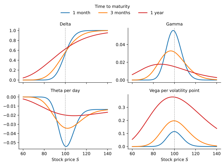
Desks quote the Greeks in units that match the moves they care about. Theta is usually reported per calendar day, \Theta/365, or per trading day, \Theta/252. Vega is reported per volatility point, \mathcal{V}/100, the change in value when implied volatility rises from, say, 20% to 21%. Delta is often reported in dollars, S \Delta, the dollar exposure equivalent to the position in the stock, and gamma as the profit from a 1% move in the stock, \frac{1}{2} \Gamma S^{2} (0.01)^{2}.
Figure 5 plots the Greeks of a call in these units, for three maturities. Gamma and theta concentrate around the strike as expiration approaches: at the strike, the gamma of the one-month call is more than three times that of the one-year call, and the one-month call loses about 5 cents a day against 2 cents for the one-year call. A desk hedging a short-dated option near the strike must therefore trade large amounts of stock whenever the price crosses it, the risk traders call pin risk. In the limit the spike becomes infinitely tall and thin. Since delta rises from 0 to 1 as the stock price goes from zero to infinity, the area under gamma is always one, and as maturity shrinks that unit area piles up at the strike: gamma converges to a Dirac delta at K, the second derivative of the payoff \max(S - K, 0). Vega behaves the other way, and the one-year call has more than three times the vega of the one-month call. This is the pattern behind the earlier remark that gamma risk dominates for short maturities and vega risk for long ones.
Practice Problems
Problem 1 What does it mean to assert that the delta of a call option is 0.7? How can a short position in 1,000 options be made delta neutral when the delta of each option is 0.7?
Solution
It means that you need 0.7 shares to hedge every call that you write. To achieve a delta neutral position when you short 1,000 options, you need to purchase 700 shares of stock.Problem 2 Calculate the delta of an at-the-money six-month European call option on a non-dividend paying stock when the risk-free interest rate is 10% per annum and the stock price volatility is 25% per annum.
Solution
Note that \ln(S/K) = \ln(1) = 0 when S=K, i.e. for an at-the-money option. Therefore, \begin{aligned} d_{1} & = \frac{(0.10 + 0.5 (0.25)^{2})(6/12)}{0.25\sqrt{6/12}} = 0.3712 \\ \Delta & = \operatorname{Φ}(d_{1}) = 0.645 \end{aligned}Problem 3 What does it mean to assert that the theta of an option position is -0.1 when time is measured in years? If a trader feels that neither a stock price nor its implied volatility will change, what type of option position is appropriate?
Solution
Assuming that there are 252 trading days per year, a theta of -0.1 means that the position loses about 0.1/252 = \$0.0004, or 0.04 cents, per trading day if everything else stays constant. A trader who expects neither the stock price nor its implied volatility to change wants a position with positive theta, which for a delta-neutral position means negative gamma, such as a short straddle.Problem 4 What is meant by the gamma of an option position? What are the risks in the situation where the gamma of a position is large and negative and the delta is zero?
Solution
The gamma measures how the delta reacts to changes in the spot price. The risks in the situation where the gamma of a position is large and negative and the delta is zero are:
- If gamma is large in absolute terms, delta is highly sensitive to the price of the underlying asset. It is then quite risky to leave a delta-neutral portfolio unchanged for any length of time.
- For a delta neutral portfolio, if gamma is negative, theta tends to be positive and the portfolio increases in value if there is no change in S but decreases in value if there is a large positive or negative change in S.
Problem 5 Suppose that a stock price is currently $20 and that a call option with an exercise price of $25 is created synthetically using a continually changing position in the stock. Consider the following two scenarios:
- Stock price increases steadily from $20 to $35 during the life of the option
- Stock price oscillates wildly, ending up at $35
Which scenario would make the synthetically created option more expensive? Explain your answer.
Solution
Scenario b. The cost of delta hedging is driven by gamma: each rebalancing trade buys after the price rises and sells after it falls, losing an amount proportional to \frac{1}{2}\Gamma(\Delta S)^{2}. In scenario b. the stock oscillates widely, generating many large moves and therefore higher total hedging costs, even though the final stock price is the same in both cases.Problem 6 A financial institution has the following portfolio of over-the-counter options on the euro:
| Type | Position | Delta of option | Gamma of option | Vega of option |
|---|---|---|---|---|
| Call | -1,000 | 0.5 | 2.2 | 1.8 |
| Call | -500 | 0.8 | 0.6 | 0.2 |
| Put | -2,000 | -0.4 | 1.3 | 0.7 |
| Call | -500 | 0.7 | 1.8 | 1.4 |
A traded option is available with a delta of 0.6, a gamma of 1.5, and a vega of 0.8. Please answer the following:
- What position in the traded option and the euro, would make the portfolio both gamma neutral and delta neutral?
- What position in the traded option and the euro, would make the portfolio both vega neutral and delta neutral?
- Suppose that a second traded option with a delta of 0.1, a gamma of 0.5, and a vega of 0.6 is available. How could the portfolio be made delta, gamma, and vega neutral?
Solution
The delta and gamma of the existing portfolio are: \begin{aligned} \Delta & = -1{,}000(0.5) - 500(0.8) - 2{,}000(-0.4) - 500(0.7) = -450 \\ \Gamma & = -1{,}000(2.2) - 500(0.6) - 2{,}000(1.3) - 500(1.8) = -6{,}000 \end{aligned} To make the portfolio gamma neutral, we need to buy N = 6{,}000 / 1.5 = 4{,}000 new options with a gamma of 1.5 each. The resulting delta is \Delta = -450 + 4{,}000 \times 0.6 = 1{,}950, that can be hedged by borrowing and selling €1,950.
The vega of the existing portfolio is: \mathcal{V} = -1{,}000(1.8) - 500(0.2) - 2{,}000(0.7) - 500(1.4) = -4{,}000.
To make the portfolio vega neutral, we need to buy N = 4{,}000 / 0.8 = 5{,}000 new options with a vega of 0.8 each. The resulting delta is \Delta = -450 + 5{,}000(0.6) = 2{,}550, that can be hedged by borrowing and selling €2,550.
Let N_{1} denote the number of options with delta of 0.6, a gamma of 1.5, and a vega of 0.8, and N_{2} denote the number of options with delta of 0.1, a gamma of 0.5, and a vega of 0.6. Then we must solve: \begin{aligned} 1.5 N_{1} + 0.5 N_{2} & = 6{,}000 \\ 0.8 N_{1} + 0.6 N_{2} & = 4{,}000 \end{aligned} This yields N_{1} = 3{,}200 and N_{2} = 2{,}400. The resulting delta is equal to \Delta = -450 + 3{,}200 \times 0.6 + 2{,}400 \times 0.1 = 1{,}710, that can be hedged by borrowing and then selling €1,710.
Problem 7 Which of the following options strategies have negative theta? Assume that all options are European and written on an asset that does not pay dividends and that the risk-free rate is positive. Select all alternatives that are correct.
- A long straddle with a strike price equal to the current stock price.
- A long strangle with strike prices K_{1} < K_{2} in which the current stock price is between K_{1} and K_{2}.
- A bull spread with strike prices K_{1} < K_{2} in which the current stock price is less than K_{1}.
- A bear spread with strike prices K_{1} < K_{2} in which the current stock price is less than K_{1}.
Solution
Alternatives a., b. and c. are correct.Problem 8 Consider a butterfly strategy with strike prices K_{1} < K_{2} < K_{3} that you made using European call options written on a non-dividend-paying asset. The risk-free rate is 5% per year. In which scenarios will the gamma of the butterfly be negative? Select all that apply.
- The current stock price is equal to K_{1}.
- The current stock price is equal to K_{2}.
- The current stock price is equal to K_{3}.
- The gamma of a butterfly is never negative.
Solution
Only alternative b. is correct.Problem 9 Consider a bull spread that you made by buying a European call with a strike K_{1} and selling a European call with a strike K_{2}, where K_{1} < K_{2}. Both options are written on a non-dividend-paying asset. The risk-free rate is 5% per year. Which alternative is correct?
- The delta of the bull spread is always positive.
- The delta of the bull spread is always negative.
- The delta of the bull spread is negative if the stock price is less than K_{1} and positive otherwise.
- The delta of the bull spread is positive if the stock price is less than K_{1} and negative otherwise.
Solution
Since the bull-spread is a bullish bet on the stock, its delta is always positive.Problem 10 Which of the following instruments and/or strategies have a gamma equal to zero? Select all that apply.
- A risk-free zero-coupon bond.
- A long call and a long put with the same strike.
- A stock.
- A long call and a short put with the same strike.