The Black-Scholes Model

The Black-Scholes formula is one of the most celebrated results in finance. In this chapter we show how to replicate the payoff of a European call or put option written on a non-dividend paying stock by dynamically trading in the stock and a risk-free bond. The replication strategy is self-financing, and therefore determines the no-arbitrage price of the option.

A key byproduct of the replication strategy is that the partial differential equation (PDE) that characterizes the price of the option does not depend on the real dynamics of the stock. We could obtain the same pricing equation regardless of the risk premium investors demand. This suggests a powerful idea to price the option. Let us assume that all investors are risk-neutral. If this was the case, the replication argument that gives the correct price of the option would still hold. However, in such a world, all assets should be priced by discounting their payoffs at the risk-free rate.

The risk-neutral approach provides us with a simpler way to derive the Black-Scholes formula. Since the risk-neutral dynamics of the non-dividend paying stock are driven by a GBM with drift equal to the risk-free rate, the stock price at maturity is log-normally distributed, which allows us to apply the formulas for partial expectations in order to price the option.

The Replicating Portfolio Approach

In order to price a call or put option, we take the point of view of a trading desk that makes the market for option contracts. Their sales team just sold a European option H written on a non-dividend paying stock S with maturity T to a client. At this point, the traders of the desk are in charge of hedging the exposure of the short position.

The Traders’ Problem

Since the option depends on the stock, it makes sense to try to hedge the exposure by trading dynamically in the stock and a risk-free bond. Specifically, we will try to replicate the option by buying (or selling) N_{S, t} units of the stock and N_{Z, t} units of a zero-coupon bond with face value K and maturity T, respectively, at each time t \leq T.¹ If we call V the value of such replicating portfolio, we have that at time t < T: V_{t} = N_{S, t} S_{t} + N_{Z, t} Z_{t}.

¹ To simplify notation, I will suppress the dependence on time whenever there is no ambiguity.

In order to replicate the option, we want to make sure that the value of the portfolio at time t = T equals the payoff of the derivative, that is: V_{T} = F(S_{T}).

For example, if we consider a European call option then F(S_{T}) = \max(S_{T} - K, 0), whereas for a European put option we have that F(S_{T}) = \max(K - S_{T}, 0).

At time t+\Delta t, the value of the replicating portfolio is: V_{t + \Delta t} = N_{S, t} S_{t + \Delta t} + N_{Z, t} Z_{t + \Delta t}, which implies that: \Delta V_{t} = N_{S, t} \Delta S_{t} + N_{Z, t} \Delta Z_{t}. The change in value comes only from price changes, because the positions chosen at t are held until t + \Delta t. At that date the portfolio is rebalanced to new positions N_{S, t + \Delta t} and N_{Z, t + \Delta t}, paid for entirely with its current value, so that no money is added or withdrawn. A strategy with this property is self-financing, exactly as in the dynamic replication of Multiple Periods.

As \Delta t \rightarrow 0, we have that: \begin{aligned} dV & = N_{S} dS + N_{Z} dZ \\ & = N_{S} dS + N_{Z} (r Z dt) \\ & = N_{S} dS + (N_{Z} Z) r dt, \end{aligned} \tag{1} where in the second line we used the fact that dZ = r Z dt.²

² Note that if Z = K e^{-r (T - t)}, then dZ = r K e^{-r (T - t)} dt = r Z dt.

Now, the replication works in the following way. We determine first how many shares of the stock to buy or sell, depending on whether the option is a call or put. Then, given the number of shares that we need to hold and the value of the portfolio at time t, we see how much money we need to borrow or invest at the risk-free rate to keep our portfolio self-financing.

The amount invested in the risk-free bonds is such that N_{Z} Z = V - N_{S} S, meaning the bond position absorbs whatever remains after the stock position is funded. Thus, if we replace N_{Z} Z in (1) we get that dV = r (V - N_{S} S) dt + N_{S} dS. \tag{2} Equation (2) captures the dynamics of the replicating portfolio needed to hedge the option that the trading desk just sold. As such, it represents the dynamics of the long position that the desk will hold to offset the risk of the short position. Thus, this is a classical long-short strategy. If the hedge is successful, the dynamics of both legs must also be the same.

The Sales Team Problem

As mentioned before, the sales team just sold a European option H written on a non-dividend paying stock S with maturity T to a client. Since our objective is to make sure that the value of the derivative equals that of the replicating portfolio, let us also call V the value of the derivative, abusing notation slightly. If we assume that V = V(S,t) is a smooth function of S and t, then Itô’s lemma implies that: \begin{aligned} dV & = \frac{\partial V}{\partial S} dS + \frac{1}{2} \frac{\partial^{2} V}{\partial S^{2}} (dS)^{2} + \frac{\partial V}{\partial t} dt \\ & = \frac{\partial V}{\partial S} dS + \frac{1}{2} \sigma^{2} S^{2} \frac{\partial^{2} V}{\partial S^{2}} dt + \frac{\partial V}{\partial t} dt, \end{aligned} where in the second line we have used the fact that (dS)^{2} = \sigma^{2} S^{2} dt. We can arrange the previous expression so that: dV = \left(\frac{1}{2} \sigma^{2} S^{2} \frac{\partial^{2} V}{\partial S^{2}} + \frac{\partial V}{\partial t}\right) dt + \frac{\partial V}{\partial S} dS. \tag{3} Equation (3) captures the dynamics of the short position.

Getting the Hedge to Work

We want to make sure that the hedge works so that the changes in value of the option equal the changes of the replicating portfolio. Therefore, replication will succeed if we can determine N_{S} such that both dynamics are the same: \underbrace{\left(\frac{1}{2} \sigma^{2} S^{2} \frac{\partial^{2} V}{\partial S^{2}} + \frac{\partial V}{\partial t}\right) dt + \frac{\partial V}{\partial S} dS}_{\text{Changes in the value of the option}} = \underbrace{\vphantom{\left(\frac{1}{2}\right)} r (V - N_{S} S) dt + N_{S} dS}_{\text{Changes in the replicating portfolio}} \tag{4} Equation (4) shows that replication will indeed work if: N_{S} = \frac{\partial V}{\partial S}. \tag{5} This is a fundamental relationship in derivatives pricing. It states that the number of shares needed to replicate the derivative is equal its sensitivity to the underlying asset. The street name of this quantity is the delta (\Delta) of the derivative. Also, a by-product of choosing N_{S} to equal the delta of the derivative is that it really does not matter what drift we have for the stock. We will use this fact in a moment to define the risk-neutral pricing measure in continuous time.

Second, it must be the case that: \frac{1}{2} \sigma^{2} S^{2} \frac{\partial^{2} V}{\partial S^{2}} + \frac{\partial V}{\partial t} = r \left(V - S \frac{\partial V}{\partial S}\right)

Therefore: \frac{1}{2} \sigma^{2} S^{2} \frac{\partial^{2} V}{\partial S^{2}} + r S \frac{\partial V}{\partial S} + \frac{\partial V}{\partial t} - r V = 0, \tag{6} subject to V_{T} = F(S_{T}).

Equation (6) is the celebrated Black-Scholes partial differential equation (PDE) which allowed the authors to compute their influential formula in 1973! Solving PDEs, in general, is very hard so we will resort to a different approach to price European call and put options.

The Risk-Neutral Pricing Approach

The PDE (6) contains the volatility \sigma and the interest rate r, but not the expected return \mu of the stock. Replication works whatever \mu is, because holding N_{S} = \partial V / \partial S shares cancels the dS terms on both sides of (4), and with them any bet on the direction of the stock. The binomial model had the same feature: the real probability p of an up move never entered the price of an option, and the risk-neutral probability q was a pricing device implied by the price of the stock, as in the bookmaker example of Binomial Pricing. In continuous time, the expected return \mu plays the role of p.

The Drift of the Stock is Irrelevant

In our model, the stock price follows a geometric Brownian motion such that: dS = \mu S dt + \sigma S dB. \tag{7} In equilibrium, if the stock returns co-vary positively with the returns of the market, as it is the case for most stocks, the drift \mu of the stock should be greater than the risk-free rate r. Indeed, risk-averse investors would command a risk-premium to hold a risky asset that increases their exposure to the market.

Since the price of the option does not depend on \mu, it must be the same in every economy with the same volatility \sigma and interest rate r, whatever risk premium investors demand. In particular, it must be the same in an economy of risk-neutral investors, who demand no risk premium, so that every asset, including the stock, has an expected return equal to r. In that economy the stock follows dS = r S dt + \sigma S dB^{*}. \tag{8} The asterisk marks that B^{*} is a Brownian motion under the probabilities of the risk-neutral economy, not under the real ones, just as q differs from p in a binomial tree. The volatility is the same in both, since it is what replication depends on. In terms of Modeling Stock Prices, where the discounted stock price e^{-r t} S has drift \mu - r, the risk-neutral probabilities are the ones under which discounted prices have zero drift.

We can now apply Itô’s lemma to the derivative to find: \begin{aligned} dV & = \left(r S \frac{\partial V}{\partial S} + \frac{1}{2} \sigma^{2} S^{2} \frac{\partial^{2} V}{\partial S^{2}} + \frac{\partial V}{\partial t}\right) dt + \left(\sigma S \frac{\partial V}{\partial S}\right) dB^{*} \\ & = r V dt + \left(\sigma S \frac{\partial V}{\partial S}\right) dB^{*}. \end{aligned} \tag{9} Equation (9) says that if the expected return of the stock is the risk-free rate, then the expected return of any derivative written on the stock is also the risk-free rate.

This is exactly how an economy populated by risk-neutral investors looks. The expected return of any non-dividend paying asset is the risk-free rate, since risk-neutral investors, by definition, do not care about risk and hence do not command a risk premium to hold risky assets in their portfolios.

With this insight, the valuation of the derivative is simple. In a risk-neutral world, the value of any risky asset is equal to its expected payoff discounted at the risk-free rate, V = e^{-r T} \operatorname{E}^{*}(F(S_{T})). \tag{10} Therefore, to value a European call or put option, all we need to do is compute the expected payoff assuming that the drift of the stock equals r, and then discount the expected payoff at the risk-free rate.

Equation (10) presents an alternative approach to compute the price of a derivative without having to solve the PDE defined in (6). Nevertheless, the risk-neutral approach is valid because we were able to replicate the derivative in the first place by trading in the stock and the risk-free bond.

Pricing a European Call Option

We can now use (10) to compute the premium of a European call option written on a non-dividend paying stock with maturity T and strike price K. The price of the call should then be C = e^{-r T} \operatorname{E}^{*}\left((S_{T} - K) 1\kern-0.25em\text{l}_{\{S_{T} > K\}} \right) = e^{-r T} \operatorname{E}^{*}\left(S_{T} 1\kern-0.25em\text{l}_{\{S_{T} > K\}} \right) - e^{-r T} \operatorname{E}^{*}\left(K 1\kern-0.25em\text{l}_{\{S_{T} > K\}} \right). Under the risk-neutral probabilities the stock follows (8), a GBM with expected return r. Solving it as in Modeling Stock Prices shows that \ln(S_{T}) \sim \mathcal{N}(m, s^{2}), with m = \ln(S) + \left(r - \tfrac{1}{2} \sigma^{2}\right) T, \qquad s = \sigma \sqrt{T}. The partial expectations of a lognormal random variable then apply with d = (m - \ln(K)) / s and d + s in place of d + \sigma. These are the two quantities \begin{aligned} d_{2} & = \frac{m - \ln(K)}{s} = \frac{\ln(S/K) + (r - \frac{1}{2} \sigma^{2}) T}{\sigma \sqrt{T}}, \\ d_{1} & = d_{2} + \sigma \sqrt{T} = \frac{\ln(S/K) + (r + \frac{1}{2} \sigma^{2}) T}{\sigma \sqrt{T}}, \end{aligned} and since \operatorname{E}^{*}(S_{T}) = e^{m + \frac{1}{2} s^{2}} = S e^{r T}, \operatorname{E}^{*}\left(S_{T} 1\kern-0.25em\text{l}_{\{S_{T} > K\}} \right) = S e^{r T} \operatorname{Φ}(d_{1}), \qquad \operatorname{E}^{*}\left(K 1\kern-0.25em\text{l}_{\{S_{T} > K\}} \right) = K \operatorname{Φ}(d_{2}). \tag{11} Discounting both terms at the risk-free rate gives the Black-Scholes formula for a European call, C = S \operatorname{Φ}(d_{1}) - K e^{-r T} \operatorname{Φ}(d_{2}).

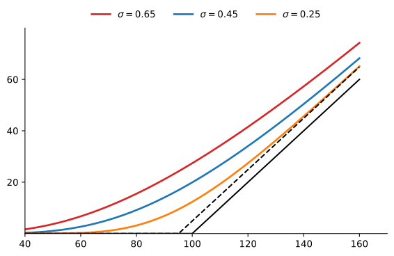
Let’s see how the call price varies with different values of the stock price.

Figure 1: The figure plots the Black-Scholes call premium C(S) if r=0.05, \sigma=0.45, T=1 and K=100. It also shows the call option payoff given by \max(S - K, 0) and the lower bound for a European call given by \max(S - K e^{-r T}, 0).

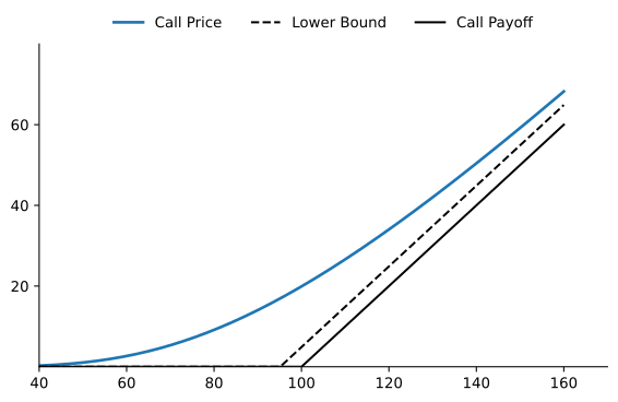
The figure above shows that the call premium is an increasing function of the stock price, keeping everything else constant. This makes sense since for a given strike price, a higher stock price implies that the call is closer to or deeper in-the-money. In other words, the derivative of the call price with respect to the stock price must be positive. The graph also shows that the function is convex, meaning that the second derivative of the call price with respect to the stock price is also positive.

Call Delta

Practitioners usually call the number of shares required to make the replication work the call delta. Equation (5) shows that the number of shares N_{S} required to hedge the European call is the partial derivative of the call price with respect the current stock price. Now that we have an expression for the call price, we can compute the call delta explicitly.

WarningCall Delta

In the Black-Scholes model, the delta of the European call is given by: \frac{\partial C}{\partial S} = \operatorname{Φ}(d_{1}). \tag{12}

Proof

We need to differentiate C with respect to S. Note that d_{1} and d_{2} are also functions of S: \begin{aligned} \frac{\partial C}{\partial S} & = \frac{\partial \left(S \operatorname{Φ}(d_{1})\right)}{\partial S} - K e^{-r T} \frac{\partial \operatorname{Φ}(d_{2})}{\partial S} \\ & = \operatorname{Φ}(d_{1}) + S \frac{\partial \operatorname{Φ}(d_{1})}{\partial S} - K e^{-r T} \frac{\partial \operatorname{Φ}(d_{2})}{\partial S} \\ & = \operatorname{Φ}(d_{1}) + S \mathop{\Phi^{'}}(d_{1}) \frac{\partial d_{1}}{\partial S} - K e^{-r T} \mathop{\Phi^{'}}(d_{2}) \frac{\partial d_{2}}{\partial S} \\ & = \operatorname{Φ}(d_{1}) + \underbrace{\left(S \mathop{\Phi^{'}}(d_{1}) - K e^{-r T} \mathop{\Phi^{'}}(d_{2})\right)}_{=0} \frac{1}{S \sigma \sqrt{T}} \\ & = \operatorname{Φ}(d_{1}), \end{aligned} where in the fourth line we used Equation (14).

The call delta is then the slope coefficient of the call price with respect to the stock price. Because \operatorname{Φ}(d_{1}) > 0, the function C(S) must be increasing in S.

Figure 2: The figure plots the Black-Scholes call premium C(S) where r = 0.05, \sigma = 0.45, T = 1 and K = 100, and shows the tangent line at S = 100 whose slope coefficient is the delta of the call given by \operatorname{Φ}(d_{1}).

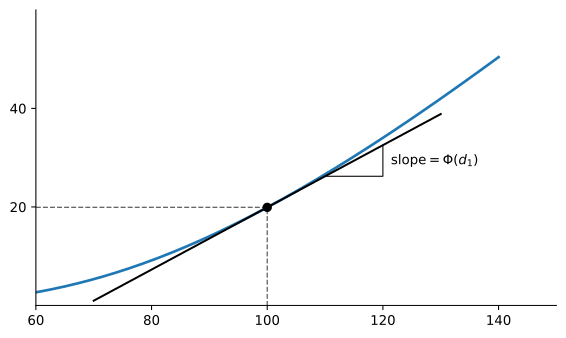
Therefore, the delta of the call measures how sensitive the call premium is to small changes in the stock price. This is exactly why the trader needs to hold delta shares of the stock to hedge the risk of the short call position.

Finally, we have that for a European call option: C = N_{S} S + N_{Z} Z = S \operatorname{Φ}(d_{1}) - K e^{-r T} \operatorname{Φ}(d_{2}) which because of (12) implies that: N_{Z} = -\operatorname{Φ}(d_{2})

Therefore, to replicate a European call option we need to go long \operatorname{Φ}(d_{1}) shares of stock and short \operatorname{Φ}(d_{2}) risk-free bonds with face value K and maturity T. The call can then be seen as a levered position in the underlying asset. Also, note that since 0<\operatorname{Φ}(d_{1})<1, the delta of the call for a non-dividend-paying asset is bounded between 0 and 1. As we saw in the previous figure, for a given spot price, the delta of the call represents the slope coefficient of the tangency line at that point.

Pricing a European Put Option

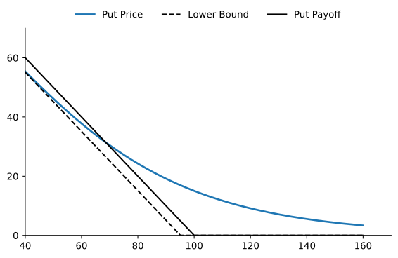
Consider now a European put option with the same characteristics as the previous call. According to put-call parity, it must be the case that: C - P = S - K e^{-r T}

Hence, \begin{aligned} P & = C - (S - K e^{-rT}) \\ & = S \operatorname{Φ}(d_{1}) - K e^{-r T} \operatorname{Φ}(d_{2}) - (S - K e^{-rT}) \\ & = K e^{-r T} (1 - \operatorname{Φ}(d_{2})) - S (1 - \operatorname{Φ}(d_{1})) \\ & = K e^{-r T} \operatorname{Φ}(-d_{2}) - S \operatorname{Φ}(-d_{1}). \end{aligned}

Example 1 Consider a non-dividend paying stock that currently trades for $100. The risk-free rate is 4% per year, continuously compounded and constant for all maturities. The instantaneous volatility of returns is 25% per year. Consider at-the-money call and put options written on the stock with maturity 9 months. Then, \begin{aligned} d_{1} & = \frac{\ln(100/100) + (0.04 + 0.5(0.25)^{2})(0.75)}{0.25\sqrt{0.75}} = 0.2468, \\ d_{2} & = 0.2468 - 0.25\sqrt{0.75} = 0.0303. \end{aligned} Therefore, \operatorname{Φ}(d_{1}) = 0.5975 and \operatorname{Φ}(d_{2}) = 0.5121, which implies that: \begin{aligned} C & = 100 \times 0.5975 - 100e^{-0.04 \times 0.75} \times 0.5121 = \$10.05, \\ P & = 100e^{-0.04(0.75)} \times (1 - 0.5121) - 100 \times (1 - 0.5975) = \$7.10. \\ \end{aligned}

Figure 3: The figure plots the Black-Scholes put premium P(S) if r = 0.05, \sigma = 0.45, T = 1 and K = 100. It also shows the put option payoff given by \max(K - S, 0) and the lower bound for a European put given by \max(K e^{-r T} - S, 0).

Put Delta

We can use put-call parity to compute N_{S} for the put: \begin{aligned} N_{S} & = \frac{\partial P}{\partial S} \\ & = \frac{\partial (C - S + K e^{-rT})}{\partial S} \\ & = \operatorname{Φ}(d_{1}) - 1 \\ & = -\operatorname{Φ}(-d_{1}) < 0. \end{aligned}

Figure 4: The figure plots the Black-Scholes put premium P(S) where r = 0.05, \sigma = 0.45, T = 1 and K = 100, and shows the tangent line at S = 100 whose slope coefficient is the delta of the put given by -\operatorname{Φ}(-d_{1}) = \operatorname{Φ}(d_{1}) - 1.

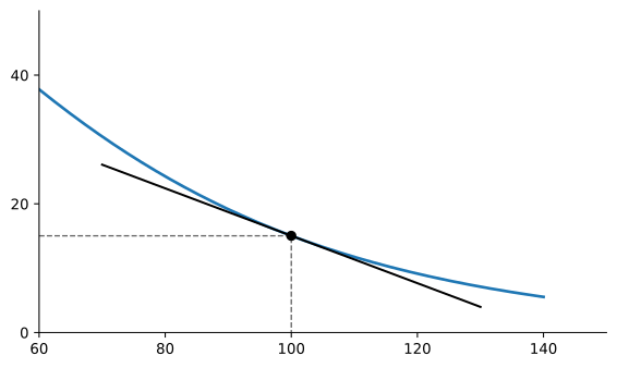
The fact that we also have P = N_{S} S + N_{Z} Z implies that: N_{Z} = \operatorname{Φ}(-d_{2}) > 0. Therefore, to replicate a European put option, we need to go short \operatorname{Φ}(-d_{1}) shares of stock and long \operatorname{Φ}(-d_{2}) risk-free bonds with face value K and maturity T.

Finishing In-The-Money

Dividing the second partial expectation in (11) by K gives the risk-neutral probability that the call ends in the money, \operatorname{P}^{*}(S_{T} > K) = \operatorname{E}^{*}\left(1\kern-0.25em\text{l}_{\{S_{T} > K\}}\right) = \operatorname{Φ}(d_{2}), which also implies \begin{aligned} \operatorname{P}^{*}(S_{T} < K) & = 1 - \operatorname{P}^{*}(S_{T} > K) \\ & = 1 - \operatorname{Φ}(d_{2}) \\ & = \operatorname{Φ}(-d_{2}). \end{aligned} Therefore, the risk-neutral probability that the call will expire in-the-money is equal to \operatorname{Φ}(d_{2}) whereas the risk-neutral probability that the put finishes in-the-money is given by \operatorname{Φ}(-d_{2}).

These are not forecasts. Under the real probabilities the stock grows at the rate \mu, and the same calculation gives \operatorname{P}(S_{T} > K) = \operatorname{Φ}\left(\frac{\ln(S/K) + (\mu - \frac{1}{2} \sigma^{2}) T}{\sigma \sqrt{T}}\right), which is larger than \operatorname{Φ}(d_{2}) when \mu > r. Like the bookmaker’s odds, risk-neutral probabilities are implied by prices, not by a view on where the stock is going.

Summary

WarningBlack-Scholes Model for a Non-Dividend Paying Stock

Consider a non-dividend paying stock S that follows a GBM under the risk-neutral measure:

dS = r S dt + \sigma S dB^{*}

The price of European call and put options with strike price K and time-to-maturity T are given by: \begin{aligned} C & = S \operatorname{Φ}(d_{1}) - K e^{-r T} \operatorname{Φ}(d_{2}), \\ P & = K e^{-r T} \operatorname{Φ}(-d_{2}) - S \operatorname{Φ}(-d_{1}), \end{aligned} where \begin{aligned} d_{1} & = \frac{\ln(S/K) + (r + \frac{1}{2} \sigma^{2}) T}{\sigma \sqrt{T}}, \\ d_{2} & = d_{1} - \sigma \sqrt{T}. \end{aligned} Furthermore, the delta of the call is given by \operatorname{Φ}(d_{1}) whereas the delta of the put is computed as -\operatorname{Φ}(-d_{1}).

Finally, the risk-neutral probability that the call will expire in-the-money is equal to \operatorname{Φ}(d_{2}) whereas the risk-neutral probability that the put finishes in-the-money is given by \operatorname{Φ}(-d_{2}).

The Impact of Volatility

One of the most important determinants of option prices in the Black-Scholes model is volatility.

WarningVega

For European call and put options we have that: \frac{\partial C}{\partial \sigma} = \frac{\partial P}{\partial \sigma} = S \mathop{\Phi^{'}}(d_{1}) \sqrt{T} > 0. \tag{13}

Proof

We start by differentiating C with respect to \sigma: \begin{aligned} \frac{\partial C}{\partial \sigma} & = S \frac{\partial \operatorname{Φ}(d_{1})}{\partial \sigma} - K e^{-r T} \frac{\partial \operatorname{Φ}(d_{2})}{\partial \sigma} \\ & = S \mathop{\Phi^{'}}(d_{1}) \frac{\partial d_{1}}{\partial \sigma} - K e^{-r T} \mathop{\Phi^{'}}(d_{2}) \frac{\partial d_{2}}{\partial \sigma} \\ & = S \mathop{\Phi^{'}}(d_{1}) \frac{\partial d_{1}}{\partial \sigma} - K e^{-r T} \mathop{\Phi^{'}}(d_{2}) \frac{\partial (d_{1} - \sigma \sqrt{T})}{\partial \sigma} \\ & = \underbrace{\left(S \mathop{\Phi^{'}}(d_{1}) - K e^{-r T} \mathop{\Phi^{'}}(d_{2})\right)}_{=0} \frac{\partial d_{1}}{\partial \sigma} + K e^{-r T} \mathop{\Phi^{'}}(d_{2}) \sqrt{T} \\ & = S \mathop{\Phi^{'}}(d_{1}) \sqrt{T}. \end{aligned} Note that because of put-call parity we also have that: \begin{aligned} C - P & = S - K e^{-r T} \Rightarrow \frac{\partial C}{\partial \sigma} - \frac{\partial P}{\partial \sigma} \\ & = 0 \Rightarrow \frac{\partial P}{\partial \sigma} = \frac{\partial C}{\partial \sigma} \\ & = S \mathop{\Phi^{'}}(d_{1}) \sqrt{T}. \end{aligned}

Hence, both European call and put options increase in value as volatility increases. Moreover, this implies that there is a one-to-one relationship between option value and volatility, i.e., we can use volatility to quote prices and vice-versa. The volatility that matches the observed price of an option is called the implied volatility.

Figure 5: The figure shows the Black-Scholes call premium for different levels of volatility where r = 0.05, T = 1 and K = 100. The dashed line represents the lower bound for the European call and the solid black line is the call payoff at maturity.

Implied Volatility

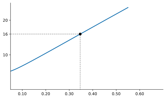
Example 2 Consider a non-dividend paying stock that currently trades for $100. The risk-free rate is 5% per year, continuously compounded and constant for all maturities. An ATM European call option written on the stock with maturity 12 months trades for $16. We can check that \sigma = 34.66\% prices the call correctly: \begin{aligned} d_{1} & = \frac{\ln(100/100) + (0.05 + 0.5(0.3466)^{2})(1)}{0.3466\sqrt{1}} = 0.3176, \\ d_{2} & = 0.3176 - 0.3466\sqrt{1} = -0.0290. \end{aligned} Therefore, \operatorname{Φ}(d_{1}) = 0.6246 and \operatorname{Φ}(d_{2}) = 0.4884, which implies that: C = 100(0.6246) - 100e^{-0.05(1)}(0.4884) = \$16.00. Therefore, a volatility of 34.66% per year gives a call price of $16.

How can we compute the implied volatility? Unfortunately, it is not possible to solve analytically for the implied volatility. For a call option, for example, it involves solving numerically for \sigma: C_{0} = C(\sigma_{\mathit{imp}})

Alternatively, we could tabulate the price of a call option for different values of \sigma (using the same parameters as the previous example):

\sigma	0.05	0.10	0.15	0.20	0.25	0.30	0.35	0.40
C	5.28	6.80	8.59	10.45	12.34	14.23	16.13	18.02

We can see that \sigma=35\% gives a call price of \$16.13, which is quite close to the true implied volatility of 34.66\%.

Figure 6: The figure shows the Black-Scholes call premium C(\sigma) as a function of \sigma where S=100, r = 0.05, T = 1 and K = 100. We can see that for C = \$16 the corresponding volatility is approximately 35%.

The Volatility Surface

In the Black-Scholes model there is only one volatility, so every option on the same stock should have the same implied volatility, whatever its strike price and maturity. Computing the implied volatility of every traded option and plotting it against moneyness K/S and maturity gives the implied volatility surface, shown on the home page of these notes. According to the model, the surface should be flat. Figure 7 shows slices of the surface for options on the S&P 500 index, averaged over 271 trading days from 2024-08-01 to 2025-08-29. Below K/S = 1 each curve uses out-of-the-money puts, and above it out-of-the-money calls, which are the most actively traded options at each strike.

Figure 7: The figure shows the average implied volatility of S&P 500 index options against moneyness K/S for four maturities, using out-of-the-money puts for K/S < 1 and out-of-the-money calls for K/S \geq 1. The dashed line marks at-the-money options. Source: OptionMetrics through WRDS.

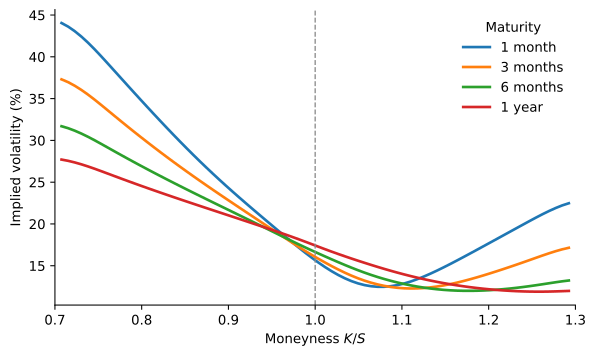
The surface is far from flat. Implied volatility falls steeply with the strike price: one-month puts struck 30% below the index trade at an implied volatility of about 44%, almost three times the 16% of at-the-money options. This pattern is called the volatility skew. It is steepest at short maturities and flattens as maturity grows, and at-the-money implied volatility rises slightly with maturity, which is called the term structure of implied volatility.

Two forces explain the skew. The first is the distribution of returns. The model assumes a lognormal price with constant volatility, but index returns have a fatter left tail, with occasional crashes, and volatility tends to rise when prices fall. Both make deep out-of-the-money puts more valuable than a lognormal distribution says, and expressing their prices with the Black-Scholes formula requires a higher \sigma. The second is that replication is imperfect in practice: trading is not continuous, prices jump, and volatility changes. Market makers who sell options therefore keep some risk they cannot hedge. Investors are net buyers of index puts, which protect their portfolios against crashes, and market makers charge for the risk they bear, so index puts are expensive relative to the model (Garleanu et al. 2009).

Garleanu, Nicolae, Lasse Heje Pedersen, and Allen M. Poteshman. 2009. “Demand-Based Option Pricing.” Review of Financial Studies 22 (10): 4259–99.

Practitioners nevertheless use the Black-Scholes formula every day, as a translation device. Traders quote option prices as implied volatilities, which can be compared across strikes, maturities, and underlying assets, and they read the price of an option that does not trade from the surface. The surface, not a single \sigma, is the object a trading desk works with.

Appendix

In this section we present a useful result that will allow us to prove the formula for the \Delta and \Gamma for European call and put options.

Indeed, we have that: \begin{aligned} (d_{2})^{2} & = (d_{1} - \sigma \sqrt{T})^{2} \\ & = (d_{1})^{2} - 2 d_{1} \sigma \sqrt{T} + \sigma^{2} T \\ & = (d_{1})^{2} - 2(\ln(S/K) + (r + \tfrac{1}{2} \sigma^{2})T) + \sigma^{2} T \\ & = (d_{1})^{2} - 2(\ln(S/K) + r T) \\ \end{aligned} Hence, \begin{aligned} \mathop{\Phi^{'}}(d_{2}) & = \frac{1}{\sqrt{2\pi}} e^{-\frac{1}{2} (d_{2})^{2}} \\ & = \frac{1}{\sqrt{2\pi}} e^{-\frac{1}{2} \left((d_{1})^{2} - 2(\ln(S/K) + r T)\right)} \\ & = \frac{S}{K} e^{r T} \mathop{\Phi^{'}}(d_{1}) \\ \end{aligned} which implies, S \mathop{\Phi^{'}}(d_{1}) = K e^{-r T} \mathop{\Phi^{'}}(d_{2}). \tag{14}

Practice Problems

Problem 1 What is the price of a European put option on a non-dividend-paying stock when the stock price is $69, the strike price is $70, the risk-free interest rate is 5% per annum, the volatility is 35% per annum, and the time to maturity is six months?

Solution

We have that: \begin{aligned} d_{1} & = \frac{\ln(69/70) + (0.05 + \frac{1}{2}0.35^{2})(6/12)}{0.35\sqrt{6/12}} = 0.1666 \Rightarrow \operatorname{Φ}(-d_{1}) = 0.434 \\ d_{2} & = 0.1666 - 0.35\sqrt{6/12} = -0.0809 \Rightarrow \operatorname{Φ}(-d_{2}) = 0.532 \end{aligned} Hence, P = 70 e^{-0.05 (6/12)} \operatorname{Φ}(-d_{2}) - 69 \operatorname{Φ}(-d_{1}) = \$6.40.

Problem 2 A call option on a non-dividend-paying stock has a market price of $2.61. The stock price is $15, the exercise price is $13, the time to maturity is three months, and the risk-free interest rate is 5% per annum. What is the implied volatility?

Solution

We need to solve numerically 2.61 = 15 \operatorname{Φ}(d_{1}) - 13 e^{-0.05 (3/12)} \operatorname{Φ}(d_{2}), where \begin{aligned} d_{1} & = \frac{\ln(15/13) + (0.05 + \frac{1}{2} \sigma^{2})(3/12)}{\sigma\sqrt{3/12}} \\ d_{2} & = d_{1} - \sigma\sqrt{3/12} \end{aligned} Using for example Excel’s solver we find that \sigma_{\text{imp}} = 45\%.

Problem 3 Consider an option on a non-dividend-paying stock when the stock price is $30, the exercise price is $29, the risk-free interest rate is 5%, the volatility is 25% per annum, and the time to maturity is four months.

1. What is the price of the option if it is a European call?
2. What is the price of the option if it is an American call?
3. What is the price of the option if it is a European put?
4. Verify that put-call parity holds.

Solution

1. We have that: \begin{aligned} d_{1} & = \frac{\ln(30/29) + (0.05 + \frac{1}{2}0.25^{2})(4/12)}{0.25\sqrt{4/12}} = 0.4225 \Rightarrow \operatorname{Φ}(d_{1}) = 0.664 \\ d_{2} & = 0.4225 - 0.25\sqrt{4/12} = 0.2782 \Rightarrow \operatorname{Φ}(d_{2}) = 0.610 \end{aligned} Hence, C = 30 \operatorname{Φ}(d_{1}) - 29 e^{-0.05 (4/12)} \operatorname{Φ}(d_{2}) = \$2.53.
2. The same since the asset pays no dividends and the interest rate is positive.
3. Since \operatorname{Φ}(-d_{1}) = 0.336 and \operatorname{Φ}(-d_{2}) = 0.390, so we have that P = 29 e^{-0.05 (4/12)} \operatorname{Φ}(-d_{2}) - 30 \operatorname{Φ}(-d_{1}) = \$1.05.
4. We need to compare C - P and S_{0} - K e^{-r T}: \begin{aligned} C - P & = 2.53 - 1.05 = \$1.48 \\ S_{0} - K e^{-r T} & = 30 - 29 e^{-0.05 (4/12)} = \$1.48 \end{aligned}

Problem 4 Consider a European call option expiring in 6 months and with strike price equal to $38 on a non-dividend paying stock that currently trades for $40. Interestingly, the volatility of the stock is zero. If the risk-free rate is 6% per year with continuous compounding, what is the price of the option?

Solution

Since the volatility of the asset is zero, its dynamics are given by: \frac{dS}{S} = r dt which implies that S_{T} = S_{0} e^{r T}. Therefore, we know for sure if the option will finish in or out-of-the-money. In our case we have that: S_{T} = 40 e^{0.06 \times 6/12} = 41.22. Therefore, the option will finish in the money at which point we will get 41.22 - 38 = 3.22, which implies that the value of the option today is 3.22 e^{-0.06 \times 6/12} = 3.12.

Problem 5 Consider a European call option expiring in 6 months and with strike price equal to $42 on a non-dividend paying stock that currently trades for $40. Interestingly, the volatility of the stock is zero. If the risk-free rate is 6% per year with continuous compounding, what is the price of the option?

Solution

We saw in Exercise 4 that when the stock has no volatility then the price at maturity is known and equal to 41.22 < 42. The option will therefore expire out-of-the-money and its value is therefore equal to zero.

Problem 6 Consider a European put option expiring in 9 months and strike price $102 written on a non-dividend paying stock. The risk-free rate is 8% per year with continuous compounding and the stock price is $100. What is the minimum price for the put that would allow you to compute its implied volatility?

Solution

To solve the problem we need to compute the lower bound for the put price: P \geq \max(102 e^{-0.08 \times 9/12} - 100, 0) = \max(-3.94, 0) = 0 Therefore, any positive price will yield in this case an implied volatility.

Problem 7 Suppose that the sales team of a trading desk just sold a European call option contract, that is 100 European call options, to an important client. The contract is written on a non-dividend paying stock that trades for $210, expires in two years and has a strike price of $215. The risk-free rate is 6% per year with continuous compounding. A trader of the desk estimate that the volatility of the stock returns is 45% and expected to remain constant for the life of the contract.

1. How many shares of the stock does the trader need to buy/sell initially in order to hedge the exposure created by the sale of the contract?
2. How many risk-free bonds with face value $215 and expiring in two years does the trader need to buy/sell in order to make sure that the strategy is self-financing?

Solution

1. The number of shares that the trader needs to buy is equal to N_{S} = 100 \times \operatorname{Φ}(d_{1}) where: d_{1} = \frac{\ln(210/215) + (0.06 + 0.5 (0.45)^{2}) \times 2}{0.45 \sqrt{2}} = 0.4698 Therefore, the trader needs to purchase 100 \times \operatorname{Φ}(0.4698) = 68.07 shares of the stock.
2. The number of bonds that the trader needs to sell in order to keep the portfolio self-financing is 100 \times \operatorname{Φ}(d_{2}), so that N_{Z} = -100 \times \operatorname{Φ}(d_{2}), where d_{2} = 0.4698 - 0.45 \sqrt{2} = -0.1666. Therefore, the trader needs to sell 100 \times \operatorname{Φ}(-0.1666) = 43.38 risk-free bonds with face-value $215 and expiring in two years.

Problem 8 According to the Black-Scholes model, what is the price of a European put option on a non-dividend-paying stock when the stock price is $109, the strike price is $106, the risk-free interest rate is 8% per year, the volatility is 29% per year, and the time to maturity is 14 months?

Solution

The value of the European put is given by P = K e^{-r T} \operatorname{Φ}(-d_{2}) - S \operatorname{Φ}(-d_{1}).

Thus, \begin{aligned} d_{1} & = \frac{\ln(109/106) + (0.08 + 0.5 \times 0.29^{2}) \times (14/12)}{0.29 \sqrt{14/12}} = 0.5437 \\ \operatorname{Φ}(-d_{1}) & = 0.2933 \\ d_{2} & = d_{1} - 0.29 \sqrt{14/12} = 0.2304 \\ \operatorname{Φ}(-d_{2}) & = 0.4089 \end{aligned} The value of the put is P = 106 e^{-0.08 \times (14/12)} \times 0.4089 - 109 \times 0.2933 = 7.51.

Problem 9 According to the Black-Scholes model, what is the price of a European call option on a non-dividend-paying stock when the stock price is $85, the strike price is $107, the risk-free interest rate is 7% per year, the volatility is 46% per year, and the time to maturity is 6 months?

Solution

The value of the European call is given by C = S \operatorname{Φ}(d_{1}) - K e^{-r T} \operatorname{Φ}(d_{2}).

Thus, \begin{aligned} d_{1} & = \frac{\ln(85/107) + (0.07 + 0.5 \times 0.46^{2}) \times (6/12)}{0.46 \sqrt{6/12}} = -0.4374 \\ \operatorname{Φ}(d_{1}) & = 0.3309 \\ d_{2} & = d_{1} - 0.46 \sqrt{6/12} = -0.7627 \\ \operatorname{Φ}(d_{2}) & = 0.2228 \end{aligned} The value of the call is C = 85 \times 0.3309 - 107 e^{-0.07 \times (6/12)} \times 0.2228 = 5.10.

Problem 10 According to the Black-Scholes model, what is the delta of a European put option on a non-dividend-paying stock when the stock price is $92, the strike price is $109, the risk-free interest rate is 6% per year, the volatility is 65% per year, and the time to maturity is 8 months?

Solution

The delta of a European put is given by -\operatorname{Φ}(-d_{1}) = \operatorname{Φ}(d_{1}) - 1. Thus, d_{1} = \frac{\ln(92/109) + (0.06 + 0.5 \times 0.65^{2}) \times (8/12)}{0.65 \sqrt{8/12}} = 0.0212, and the delta of the put is \operatorname{Φ}(0.0212) - 1 = -0.4915.