Multiple Periods

In the one-period model, a stock can move to one of two possible prices, and we price derivatives by replication or, equivalently, by computing expected payoffs under the risk-neutral probability and discounting at the risk-free rate. This document extends that framework to multiple periods by chaining one-period trees together. We first study the structure of multi-period trees and the recombination property that keeps them tractable. We then derive the backward-induction pricing formula, show how to calibrate the tree to observed volatility, develop a closed-form shortcut for European options, and extend the tree to assets that pay a dividend yield.

Binomial Trees with Multiple Periods

The power of binomial trees becomes apparent when we chain one-period trees together to build larger ones, as the following example illustrates.

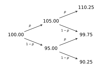
Example 1 (Two-Period Binomial Tree) The current stock price is $100. Each period, the asset can go up or down by 5% with probability p and 1 - p, respectively.

There are three possible values for the stock at the end of the tree, but four possible histories. Indeed, the price $99.75 can be reached by going up first and then down, or by going down first and then up.

Sometimes we will omit the probabilities from the diagram to keep the notation clean.

Example 2 (Four-Period Binomial Tree) The current stock price is $100. Each period the asset can go up or down by 2.5%.

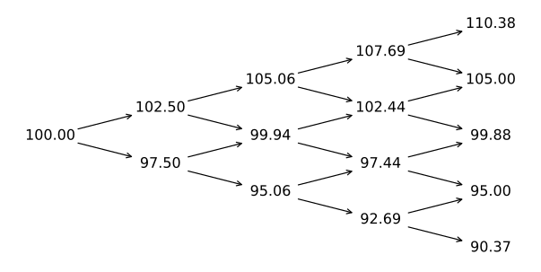
After four periods there are five possible values for the stock, one for each number of up-moves from zero to four, confirming that the tree recombines.

A key feature of the previous examples is that going up and then down yields the same price as going down and then up. When this happens we say that the tree recombines.

Recombining trees are very useful for modeling financial assets because the number of nodes grows linearly with the number of periods: after n periods there are only n + 1 possible nodes, even though the number of possible histories grows exponentially. In a non-recombining tree, by contrast, the number of nodes at period n is 2^{n}, which quickly becomes computationally prohibitive.

A sufficient condition for the tree to recombine is that the percentage increase and decrease of the stock price at each node are kept constant throughout the tree. As the following example shows, the up and down moves need not be symmetric: the tree recombines even if d \neq 1/u.

Example 3 (Recombining Trees) Is it the same for an asset to go up by 80% and then down by 30%, compared to first go down by 30% and then go up by 80%? Consider an asset whose current price is $100.

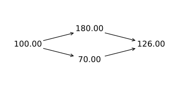
The tree recombines because of the commutative property of multiplication: S_{ud} = 100 \times 1.80 \times 0.70 = 100 \times 0.70 \times 1.80 = S_{du} In words, gaining 80% and then losing 30% is the same as first losing 30% and then gaining 80%.

The Two Period Binomial Model

We now extend the model to two periods. We would like to price a European call option with strike price K, expiring at time T and written on a non-dividend paying stock. The figure below shows the different values that we need to compute for both the stock¹ and the call option.

¹ Each period, the stock price goes up or down by u or d, respectively. Therefore, at the end of the first period we have that S_{u} = S \times u, \, S_{d} = S \times d. At the end of the second period the possible values are given by S_{uu} = S_{u} \times u, \, S_{ud} = S_{u} \times d, \, S_{dd} = S_{d} \times d. Finally, because the tree recombines, we must have that S_{ud} = S_{u} \times d = S_{d} \times u = S_{du}.

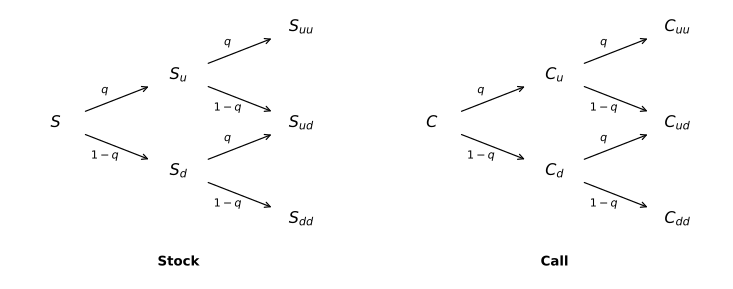
We assume that each period has equal length \Delta t = T / 2. This is not required, but it ensures that the volatility of stock returns is the same in every period. The risk-neutral probability of an up-move is then q = \frac{S e^{r \Delta t} - S d}{S u - S d} = \frac{e^{r \Delta t} - d}{u - d}. Note that the risk-neutral probability of the stock going up is the same in all nodes of the tree.

We now work backwards from expiration to the beginning of the tree. The call’s value at expiration is simply its intrinsic value: \begin{aligned} C_{uu} & = \max(S_{uu} - K, 0), \\ C_{ud} & = \max(S_{ud} - K, 0), \\ C_{dd} & = \max(S_{dd} - K, 0). \end{aligned} If the stock price goes up during the first period, the call price at that point must be equal to: C_{u} = \left( q C_{uu} + (1 - q) C_{ud} \right) e^{-r \Delta t}. Similarly, if the stock price goes down during the first period we have that: C_{d} = \left( q C_{ud} + (1 - q) C_{dd} \right) e^{-r \Delta t}. Finally, the value of the option at the beginning of the tree follows from the same one-period argument. Over the first period, the call is worth C_{u} if the stock goes up and C_{d} if it goes down. This is a two-state payoff on the stock, which we can replicate as before, so C = \left( q C_{u} + (1 - q) C_{d} \right) e^{-r \Delta t}.

The replicating portfolio changes as we move through the tree. Today we hold N_{S} = (C_{u} - C_{d})/(S_{u} - S_{d}) shares. If the stock goes up, we rebalance to N_{S}^{u} = (C_{uu} - C_{ud})/(S_{uu} - S_{ud}) shares, and if it goes down, to N_{S}^{d} = (C_{ud} - C_{dd})/(S_{ud} - S_{dd}) shares. No money needs to be added or withdrawn along the way: when we reach a node, the portfolio is worth exactly C_{u} or C_{d}, which is what the new replicating portfolio costs. The strategy is self-financing, and holding it from today replicates the call at expiration. Replication in a multi-period tree is therefore dynamic: the hedge must be adjusted every period as the stock price moves.

Example 4 (Pricing a European Call Option) The current stock price is $100 and it can go up or down by 5% each period. Each period represents three months, so \Delta t = 3/12 = 0.25. The risk-free rate is 6% per year with continuous compounding. We price a European call with maturity 6 months and strike $100.

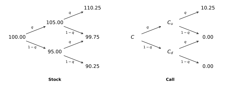
The risk-neutral probability of an up-move is then: q = \frac{e^{r \Delta t} - d}{u - d} = \frac{e^{0.06 \times 0.25} - 0.95}{1.05 - 0.95} = 0.6511.

The risk-neutral probability of a down-move is 1 - q = 0.3489. We can then compute: \begin{aligned} C_{u} & = \left( 10.25 \times q + 0 \times (1 - q) \right) e^{-0.06 \times 0.25} = \$6.57 \\ C_{d} & = \left( 0 \times q + 0 \times (1 - q) \right) e^{-0.06 \times 0.25} = \$0 \\ C & = \left( 6.57 \times q + 0 \times (1 - q) \right) e^{-0.06 \times 0.25} = \$4.22 \end{aligned} Therefore, the value of the European call is $4.22.

The hedge changes along the tree. Today the replicating portfolio holds N_{S} = (6.57 - 0)/(105 - 95) = 0.657 shares. If the stock goes up, we rebalance to N_{S}^{u} = (10.25 - 0)/(110.25 - 99.75) = 0.976 shares, since the call is then likely to finish in the money. If the stock goes down, the call can no longer pay off, and we sell all the shares: N_{S}^{d} = 0.

Example 5 (Pricing a European Put Option) We can use the risk-neutral probabilities in Example 4 to price a European put with the same characteristics. The put payoffs at expiration are \max(K - S_{T}, 0), which gives the following tree:

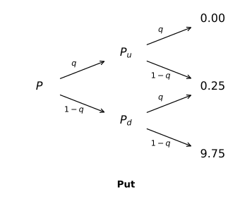
Working backwards: \begin{aligned} P_{u} & = \left( 0 \times q + 0.25 \times (1 - q) \right) e^{-0.06 \times 0.25} = \$0.09 \\ P_{d} & = \left( 0.25 \times q + 9.75 \times (1 - q) \right) e^{-0.06 \times 0.25} = \$3.51 \\ P & = \left( 0.09 \times q + 3.51 \times (1 - q) \right) e^{-0.06 \times 0.25} = \$1.26 \end{aligned}

The value of the European put can also be obtained using put-call parity. Indeed, the put is equal to a call plus a short forward: \begin{aligned} P & = C - S + K e^{-r T} \\ & = 4.22 - 100 + 100 e^{-0.06 \times 0.5} \\ & = \$1.26. \\ \end{aligned} Note that we discount the strike price using the maturity of the option which is 6 months.

Making the Tree Consistent with Observed Volatility

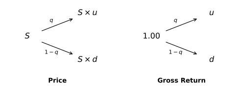
So far we have used arbitrary values for u and d. A great advantage of the binomial model is that it is possible to relate these movements to the volatility of the stock observed in the market. Over a small interval \Delta t, the choice u = e^{\sigma \sqrt{\Delta t}} and d = 1 / u produces a binomial model consistent with the Black-Scholes model of a Geometric Brownian Motion (GBM).²

² Note that in this case u \times d = 1, so the tree on average does not have a drift. The risk-neutral drift, however, is incorporated into the risk-neutral probabilities.

In other words, for small \Delta t the variance of stock returns satisfies V \approx \sigma^{2} \Delta t. Therefore, at each node the percentage change in the stock price has mean r \Delta t and variance \sigma^{2} \Delta t.

Proof

Let’s see how this modification works in a 1-period tree.

The binomial process for the stock implies that the gross return next period is either u or d with risk-neutral probability q or 1 - q, respectively. Recall that the risk-neutral probability of an up-move is: \begin{aligned} q = \frac{e^{r \Delta t} - d}{u - d}. \end{aligned} The variance of the returns over the period can then be computed as: \begin{aligned} V & = q (u - (q u + (1 - q) d))^{2} + (1 - q) (d - (q u + (1 - q) d))^{2} \\ & = q (1 - q)^{2} (u - d)^{2} + (1 - q) q^{2} (u - d)^{2} \\ & = q (1 - q) (u - d)^{2} \\ & = \left( \frac{e^{r \Delta t} - d}{u - d} \right) \left( 1 - \frac{e^{r \Delta t} - d}{u - d} \right) (u - d)^{2} \\ & = (e^{r \Delta t} - d) (u - e^{r \Delta t}) \\ & = (e^{r \Delta t} - e^{-\sigma \sqrt{\Delta t}}) (e^{\sigma \sqrt{\Delta t}} - e^{r \Delta t}). \\ \end{aligned} Therefore, \begin{aligned} \lim_{\Delta t \rightarrow 0} \frac{V}{\Delta t} & = \lim_{\Delta t \rightarrow 0} \left( \frac{e^{r \Delta t} - e^{-\sigma \sqrt{\Delta t}}}{\sqrt{\Delta t}} \right) \left( \frac{e^{\sigma \sqrt{\Delta t}} - e^{r \Delta t}}{\sqrt{\Delta t}} \right) \\ & = \lim_{\Delta t \rightarrow 0} \frac{e^{r \Delta t} - e^{-\sigma \sqrt{\Delta t}}}{\sqrt{\Delta t}} \lim_{\Delta t \rightarrow 0} \frac{e^{\sigma \sqrt{\Delta t}} - e^{r \Delta t}}{\sqrt{\Delta t}} \\ & = \sigma ^{2}. \end{aligned}

A Shortcut for European Options

In the case of European options it is possible to price a European call or put without having to work the intermediate steps. In the case of American options, however, it is necessary to check whether it is worth to exercise the option at each node of the tree. We will learn later how to handle the American option case.

Take a two-period tree. Instead of working backwards step by step, we can use the terminal payoffs directly to compute: C = \left( Q(0) C_{uu} + Q(1) C_{ud} + Q(2) C_{dd} \right) e^{-r T}, where Q(0) = q^{2}, Q(1) = 2 q (1 - q), and Q(2) = (1 - q)^{2} are the total risk-neutral probabilities of reaching each final node with zero, one or two down-moves.

We can generalize the method for an arbitrary number of periods n, which means that \Delta t = T / n. Since at each node the stock S can go up or down to S_{u} = S \times u and S_{d} = S \times d, we have that the stock price at time T can take on n + 1 different values: S_{T} = \left( \begin{array}{c} S_{T}(0) \\ S_{T}(1) \\ S_{T}(2) \\ \vdots \\ S_{T}(n - 2) \\ S_{T}(n - 1) \\ S_{T}(n) \end{array} \right) = \left( \begin{array}{c} S u ^ {n} \\ S u ^ {n - 1} d \\ S u ^ {n - 2} d ^ {2} \\ \vdots \\ S u ^ {2} d ^ {n - 2} \\ S u d ^ {n - 1} \\ S d ^ {n} \end{array} \right) The risk-neutral probability of an up-move is given by: q = \frac{e^{r \Delta t} - d}{u - d}. The total risk-neutral probability of node i = 0, \ldots, n, reached with n - i up-moves and i down-moves, is: Q(i) = \binom{n}{i} q^{n - i} (1 - q)^{i}, where \binom{n}{i} = \frac{n!}{(n - i)! i!} is a binomial coefficient. The price of European call and put options are given by: \begin{aligned} C & = e^{-r T} \sum_{i = 0}^{n}{Q(i) \max(S_{T}(i) - K, 0)} \\ P & = e^{-r T} \sum_{i = 0}^{n}{Q(i) \max(K - S_{T}(i), 0)} \end{aligned}

Pricing with Many Periods

The following example prices a European call by backward induction in a multi-period binomial tree calibrated to observed volatility, and then checks the result with the shortcut.

Example 6 (Pricing a European Call Option Using Five Periods) In this example we price a 6-month European call option with strike price $135 written on a non-dividend paying stock that currently trades at $132 and whose volatility of stock returns is 35% per year. We use an interest rate of 3% per year with continuous compounding.

We will use a 5-period binomial tree. Therefore, we have that T = 6/12 = 0.5 and \Delta t = T / 5 = 0.1, so that u = e^{0.35 \sqrt{0.1}} = 1.1170 and d = 1/1.1170 = 0.8952. The table below describes the binomial tree for the stock. For convenience, the tree is written as a lower triangle. The horizontal line describes the path where the stock price increases every period whereas the lower diagonal describes the path where the stock price goes down every period.

Time	0	0.1	0.2	0.3	0.4	0.5
Stock	132	147.45	164.71	183.98	205.52	229.57
		118.17	132.00	147.45	164.71	183.98
			105.79	118.17	132.00	147.45
				94.70	105.79	118.17
					84.78	94.70
						75.90

The risk-neutral probability of an up-move is given by: \begin{aligned} q = \frac{e^{0.03 \times 0.1} - 0.8952}{1.1170 - 0.8952} = 0.4859. \end{aligned} We can now price the call as follows.

Time	0	0.1	0.2	0.3	0.4	0.5
Call	13.16	21.23	33.18	49.79	70.92	94.57
		5.60	10.06	17.68	30.11	48.98
			1.42	2.92	6.03	12.45
				0.00	0.00	0.00
					0.00	0.00
						0.00

In the table above, the last column contains the payoffs of the call at maturity. For example, if the stock price at maturity is 229.57, then the payoff of the call is 229.57 - 135 = 94.57 which is the first number on the last column. On the other hand, if the stock price at maturity 94.70, then the call is out-of-the-money and the payoff is 0.

We work backwards on the tree by computing expected payoffs using the risk-neutral probabilities and discounting at the risk-free rate for 0.1 years. For example, the first number in the second-to-last column is computed as 70.92 = (94.57 q + 48.98 (1 - q)) e^{- 0.03 \times 0.1} where q is the risk-neutral probability computed above. We keep doing this for all nodes until we reach the beginning of the tree. The price of the call is then $13.16.

Since the call is European, the shortcut gives the same price directly from the payoffs at maturity. Only the three highest nodes pay off, so C = e^{-0.03 \times 0.5} \left( q^{5} \times 94.57 + 5 q^{4} (1 - q) \times 48.98 + 10 q^{3} (1 - q)^{2} \times 12.45 \right) = \$13.16.

A spreadsheet that shows the computations can be found here.

Assets Paying a Dividend Yield

When the asset pays a dividend yield \delta, as in The Impact of Dividends, the only change to the tree is the risk-neutral probability. Holding the asset earns the yield, so its forward price over the next period is S e^{(r - \delta) \Delta t} rather than S e^{r \Delta t}, and the risk-neutral probability must reproduce that forward price, just as in the one-period model. Say that over the next period \Delta t the asset price can go up to S_{u} = S u, or down to S_{d} = S d, and that we want to price a derivative X that pays either X_{u} or X_{d} in each state, respectively.

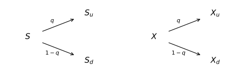
The risk-neutral probability of an up-move in this case is given by: q = \frac{e^{(r - \delta) \Delta t} - d}{u - d} The price of the derivative is then: X = (q X_{u} + (1 - q) X_{d}) e^{-r \Delta t}

The yield also changes the hedge. A share bought today grows to e^{\delta \Delta t} shares by the end of the period, so the replicating portfolio buys fewer shares up front: N_{S} = \frac{X_{u} - X_{d}}{S_{u} - S_{d}} e^{-\delta \Delta t}.

The calibration u = e^{\sigma \sqrt{\Delta t}} and d = 1/u carries over unchanged, where \sigma represents the annualized volatility of the asset returns. With several periods, we work backwards through the tree exactly as before, using this q at every node.

Example 7 Suppose that S = 110, r = 5\%, \delta = 3\%, \sigma = 30\%, K = 110, T = 9 months. Using a one-period binomial tree, let’s compute the no-arbitrage price of a European call option. The binomial trees for the asset and the call are as follows:

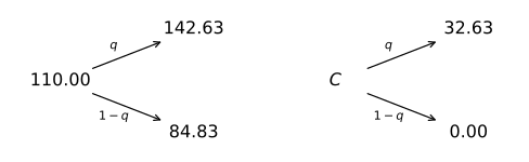
\begin{aligned} q & = \frac{110 e^{(0.05 - 0.03) \times 9/12} - 84.83}{142.63 - 84.83} = 0.4642 \\ C & = (32.63 q + 0 (1 - q)) e^{-0.05 \times 9/12} = 14.59 \end{aligned}

Practice Problems

Problem 1 A non-dividend stock trades for $100. Over each of the next two 6-month periods it is expected to go up or down by 10%. The risk-free interest rate is 8% per annum with continuous compounding.

1. What is the value of a 1-year European call option with a strike price of $100?
2. What is the value of a 1-year European put option with a strike price of $100?

Solution

1. The binomial trees for the stock and the European call are as follows:

   

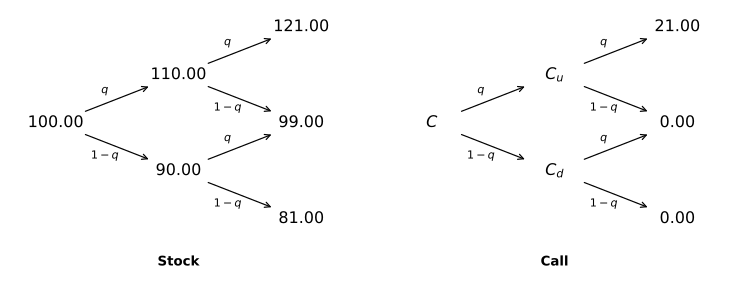
   The risk-neutral probability of an up move is: q = \frac{e^{0.08 \times 6/12} - 0.90}{1.10 - 0.90} = 0.7041. We can then compute: \begin{aligned} C_{u} & = (21 q + 0 (1 - q)) e^{-0.08 \times 6/12} = 14.21 \\ C_{d} & = (0 q + 0 (1 - q)) e^{-0.08 \times 6/12} = 0 \\ C & = (14.21 q + 0 (1 - q)) e^{-0.08 \times 6/12} = 9.61 \end{aligned}

2. The binomial tree for the European put is:

   

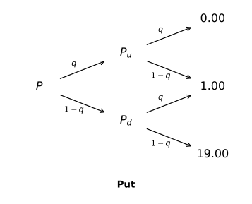
   Therefore: \begin{aligned} P_{u} & = (0 q + 1 (1 - q)) e^{-0.08 \times 6/12} = 0.28 \\ P_{d} & = (1 q + 19 (1 - q)) e^{-0.08 \times 6/12} = 6.08 \\ P & = (0.28 q + 6.08 (1 - q)) e^{-0.08 \times 6/12} = 1.92 \end{aligned}

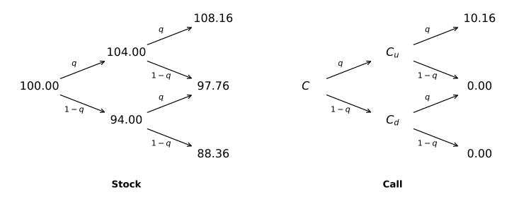
Problem 2 The current price of a non-dividend paying stock is $100. Every three months, it is expected to go up or down by 4% or 6%, respectively. The risk-free rate is 8% per year with continuous compounding. Compute the price of a European call option with strike price $98 and maturity six months written on the stock.

Solution

We have that \Delta t = 3/12, u = 1.04 and d = 0.94. The binomial trees for the stock and the European call are as follows:

The risk-neutral probability of an up move is: \begin{aligned} q = \frac{e^{0.08 \times 3/12} - 0.94}{1.04 - 0.94} = 0.8020. \end{aligned} We can then compute: \begin{aligned} C_{u} & = (10.16 q + 0 (1 - q)) e^{-0.08 \times 3/12} = 7.99 \\ C_{d} & = (0 q + 0 (1 - q)) e^{-0.08 \times 3/12} = 0 \\ C & = (7.99 q + 0 (1 - q)) e^{-0.08 \times 3/12} = 6.28 \end{aligned}

Problem 3 Consider a non-dividend paying asset for which you have the following information: S_{0} = 100, r = 4\% per year with continuous compounding, and \sigma = 20\% per year. Using a standard binomial model with four periods in which u = e^{\sigma \sqrt{\Delta t}} and d = 1/u, compute the price of an at-the-money European call option expiring in 6 months.

Solution

We start by noting that \Delta t = 0.5 / 4 = 0.125, so that u = e^{0.20 \sqrt{0.125}} = 1.0733 and d = 1 / 1.0733 = 0.9317.

The tree for the stock is:

Period	0	1	2	3	4
	100.00	107.33	115.19	123.63	132.69
		93.17	100.00	107.33	115.19
			86.81	93.17	100.00
				80.89	86.81
					75.36

The risk-neutral probability of an up-move is q = \frac{e^{0.04 \times 0.125} - 0.9317}{1.0733 - 0.9317} = 0.5177

Therefore, the tree for the call is:

Period	0	1	2	3	4
	6.29	10.27	16.19	24.13	32.69
		2.08	4.03	7.83	15.19
			0.00	0.00	0.00
				0.00	0.00
					0.00

The call is worth $6.29.

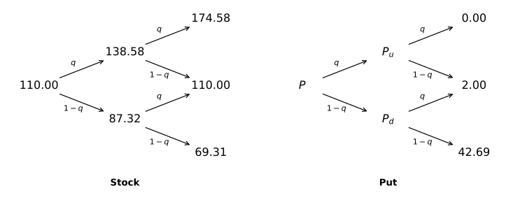
Problem 4 Suppose that S = 110, r = 4\%, \delta = 8\%, and \sigma = 40\%. Using a two-period binomial tree, compute the no-arbitrage price of a European put option with strike $112 and maturity 8 months.

Solution

First, we have that \Delta t = 4/12, which implies that u = e^{0.40 \sqrt{4/12}} = 1.2598 and d = 1/u = 0.7938. The binomial trees for the stock and the European put are as follows:

The risk-neutral probability of an up move is: q = \frac{e^{(0.04-0.08) \times 4/12} - 0.7938}{1.2598 - 0.7938} = 0.4141. We can then compute: \begin{aligned} P_{u} & = (0 q + 2 (1 - q)) e^{-0.04 \times 4/12} = 1.16 \\ P_{d} & = (2 q + 42.69 (1 - q)) e^{-0.04 \times 4/12} = 25.50 \\ P & = (1.16 q + 25.50 (1 - q)) e^{-0.04 \times 4/12} = 15.21 \end{aligned}

Problem 5 A stock that pays a dividend yield of 8% per year costs $50. Analysts estimate that there is a 50% chance that the stock trades for $60 next year if the company succeeds in developing an important vaccine. Otherwise, the stock could fall to $40. The risk-free rate is 5% per year with continuous compounding. What should be the price of a security that pays $100 next year if the stock goes up, and $0 otherwise?

Solution

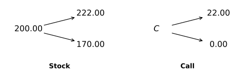
The risk-neutral probability of an up-move is: q = \frac{50 e^{0.05 - 0.08} - 40}{60 - 40} = 0.4261. The price of the security can then be computed as: X = (100 q + 0 (1 - q)) e^{-0.05} = 40.53.

Problem 6 The current price of a stock is $200. Over the next year, it is expected to go up or down by 11% or 15%, respectively. The stock pays a dividend yield of 6% per year and the risk-free rate is 7% per year with continuous compounding. A market-maker of an important investment bank just sold 100 at-the-money European call options (i.e. one contract) expiring in one year to an important client. How many shares of the stock does she need to buy in order to hedge her exposure?

Solution

The binomial trees for the stock and the call are as follows:

We need to adjust the normal hedge for the fact that the asset pays a dividend yield. In this case we have that: N_{S} = 100 \left( \frac{22 -0}{222 - 170} \right) e^{-0.06} = 39.84.

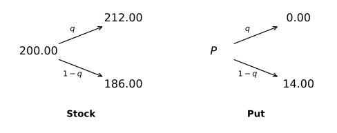
Problem 7 Consider an asset that trades for $200. Over the next six months, analysts expect that it could go up to $213 or down to $183. The asset pays a dividend yield of 7% per year. Compute the price of an at-the-money European call option expiring in six months. Assume that the risk-free rate is 9% per year with continuous compounding.

Solution

The binomial trees for the stock and the call are as follows:

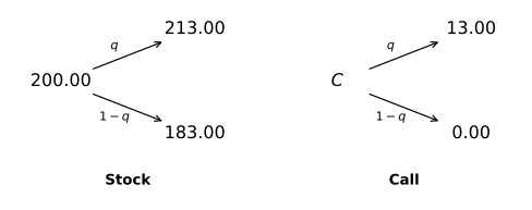
The risk-neutral probability of an up move is: q = \frac{200 e^{(0.09 - 0.07) \times 6/12} - 183}{213 - 183} = 0.6337.

We can then compute: C = (13 q + 0 (1 - q)) e^{-0.09 \times 6/12} = 7.88.

Problem 8 The current price of a stock is $100. Every three months, it is expected to go up or down by 15% or 11%, respectively. The stock pays a dividend yield of 7% per year and the risk-free rate is 8% per year with continuous compounding. Compute the price of a European call option with strike price $98 and maturity six months written on the stock.

Solution

We have that \Delta t = 3/12, u = 1.15 and d = 0.89. The binomial trees for the stock and the European call are as follows:

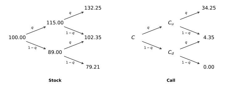
q = \frac{e^{(0.08-0.07) \times 3/12} - 0.89}{1.15 - 0.89} = 0.4327.

We can then compute: \begin{aligned} C_{u} & = (34.25 q + 4.35 (1 - q)) e^{-0.08 \times 3/12} = 16.95 \\ C_{d} & = (4.35 q + 0 (1 - q)) e^{-0.08 \times 3/12} = 1.85 \\ C & = (16.95 q + 1.85 (1 - q)) e^{-0.08 \times 3/12} = 8.21 \end{aligned}

Problem 9 Consider an asset that trades for $200. Over the next six months, analysts expect that it could go up to $212 or down to $186. The asset pays a dividend yield of 6% per year. Compute the price of an at-the-money European put option expiring in six months. Assume that the risk-free rate is 7% per year with continuous compounding.

Solution

The binomial trees for the stock and the put are as follows:

The risk-neutral probability of an up move is: q = \frac{200 e^{(0.07 - 0.06) \times 6/12} - 186}{212 - 186} = 0.5770. We can then compute: P = (0 q + 14 (1 - q)) e^{-0.07 \times 6/12} = 5.72.