The Lognormal Distribution

The Black-Scholes model assumes that the price of a stock at a future date has a lognormal distribution: its logarithm is normally distributed. This chapter collects the facts about the normal and lognormal distributions that the next chapters use. We show how to compute probabilities, the mean and standard deviation of a lognormal random variable, and the partial expectations that turn into the two terms of the Black-Scholes formula.

Why the Lognormal Distribution

Suppose a stock trades at S_{0} today and at S_{T} at a future date T. Its continuously compounded return over the period is R = \ln(S_{T} / S_{0}), so that S_{T} = S_{0} e^{R}. Split the period into many short subperiods, and let R_{1}, R_{2}, \ldots, R_{n} be the continuously compounded returns over each of them. Continuously compounded returns add up over time, R = \ln\left(\frac{S_{T}}{S_{0}}\right) = \ln\left(\frac{S_{t_{1}}}{S_{0}} \times \frac{S_{t_{2}}}{S_{t_{1}}} \times \cdots \times \frac{S_{T}}{S_{t_{n - 1}}}\right) = R_{1} + R_{2} + \cdots + R_{n}. If the returns over different subperiods are independent and none of them dominates the sum, the central limit theorem says that R is approximately normal, whatever the distribution of each R_{i}. The price S_{T} = S_{0} e^{R} is then the exponential of a normal random variable, which is what we call a lognormal random variable.

The lognormal distribution has two features that suit stock prices. A lognormal random variable is always positive, consistent with the limited liability of a stock, and its distribution is skewed to the right: a stock can at most lose all of its value, but it can gain several times its value. The binomial trees of the previous chapters already have this structure, since every period multiplies the stock price by u or d, and the logarithm of the price is a sum of independent steps.

The Normal Distribution

A random variable X is normally distributed with mean \mu and standard deviation \sigma, written X \sim \mathcal{N}(\mu, \sigma^{2}), if its probability density function (PDF) is f(x) = \frac{1}{\sqrt{2 \pi \sigma^{2}}} e^{-\frac{(x - \mu)^{2}}{2 \sigma^{2}}}. The density is the familiar bell curve, symmetric around \mu, with inflection points at \mu - \sigma and \mu + \sigma.

Figure 1: The figure shows the density function of a normally distributed random variable with mean \mu and standard deviation \sigma.

WarningMoments of the Normal Distribution

If X \sim \mathcal{N}(\mu, \sigma^{2}), then \operatorname{E}(X) = \mu and \operatorname{V}(X) = \sigma^{2}.

Proof

Let Z = (X - \mu) / \sigma, which has the standard normal density \varphi(z) = e^{-z^{2}/2} / \sqrt{2 \pi}. The function z \varphi(z) is odd, so its integral over the real line is zero and \operatorname{E}(Z) = 0. Since \varphi'(z) = -z \varphi(z), integrating by parts gives \operatorname{E}(Z^{2}) = \int_{-\infty}^{\infty} z \cdot z \varphi(z) \, dz = \Big[-z \varphi(z)\Big]_{-\infty}^{\infty} + \int_{-\infty}^{\infty} \varphi(z) \, dz = 0 + 1 = 1, so \operatorname{V}(Z) = 1. Therefore, \operatorname{E}(X) = \mu + \sigma \operatorname{E}(Z) = \mu and \operatorname{V}(X) = \sigma^{2} \operatorname{V}(Z) = \sigma^{2}.

The Standard Normal Distribution

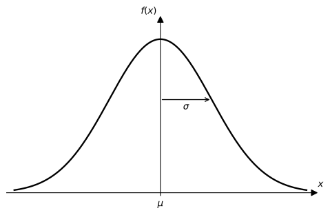
When \mu = 0 and \sigma = 1, we say that Z \sim \mathcal{N}(0, 1) has the standard normal distribution. Its cumulative distribution function (CDF) is denoted by the capital Greek letter \Phi (phi), \operatorname{Φ}(z) = \operatorname{P}(Z \leq z) = \int_{-\infty}^{z} \frac{1}{\sqrt{2 \pi}} e^{-\frac{u^{2}}{2}} \, du, the area under the density to the left of z.

Figure 2: The blue shaded area represents \operatorname{Φ}(z).

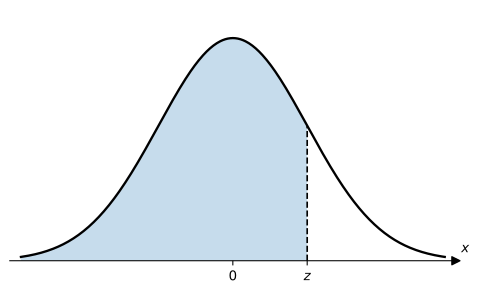
The integral has no closed form, so \operatorname{Φ}(z) is obtained from a table or a computer. In Python, SciPy computes \operatorname{Φ}(-0.4) as follows:

from scipy.stats import norm

print(norm.cdf(-0.4))

0.3445782583896758

In Excel, =norm.s.dist(-0.4,TRUE) gives the same answer.

Every normal random variable is a standard normal in disguise. If X \sim \mathcal{N}(\mu, \sigma^{2}), then its z-score Z = (X - \mu) / \sigma has the standard normal distribution, so that X = \mu + \sigma Z. We will use this representation throughout.

Computing Probabilities

To compute the probability that X is below a value x, we translate the statement into one about Z: \operatorname{P}(X \leq x) = \operatorname{P}\left(\frac{X - \mu}{\sigma} \leq \frac{x - \mu}{\sigma}\right) = \operatorname{Φ}\left(\frac{x - \mu}{\sigma}\right).

Example 1 Suppose that X \sim \mathcal{N}(\mu, \sigma^{2}) with \mu = 10 and \sigma = 25. The probability that X \leq 0 is \operatorname{P}(X \leq 0) = \operatorname{Φ}\left(\tfrac{0 - 10}{25}\right) = \operatorname{Φ}(-0.40) = 0.3446.

The probability of the whole distribution is one, so the right-tail probability is \operatorname{P}(X > x) = 1 - \operatorname{P}(X \leq x).

Figure 3: The right-tail probability is the probability of the whole distribution, which is one, minus the left-tail probability.

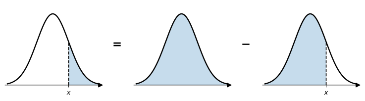
Since the standard normal density is symmetric around zero, the area to the right of z equals the area to the left of -z, so that 1 - \operatorname{Φ}(z) = \operatorname{Φ}(-z). We will use this identity to write right-tail probabilities as values of \operatorname{Φ}.

Example 2 Suppose that X \sim \mathcal{N}(\mu, \sigma^{2}) with \mu = 10 and \sigma = 25. The probability that X > 12 is \operatorname{P}(X > 12) = 1 - \operatorname{Φ}\left(\tfrac{12 - 10}{25}\right) = 1 - \operatorname{Φ}(0.08) = 1 - 0.5319 = 0.4681.

The probability that X falls in an interval (x_{1}, x_{2}] is the area to the left of x_{2} minus the area to the left of x_{1}, \operatorname{P}(x_{1} < X \leq x_{2}) = \operatorname{P}(X \leq x_{2}) - \operatorname{P}(X \leq x_{1}).

Figure 4: Subtracting the area to the left of x_{1} from the area to the left of x_{2} gives the probability that x_{1} < X \leq x_{2}.

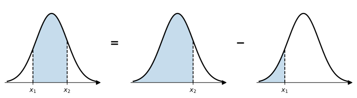
Example 3 Suppose that X \sim \mathcal{N}(\mu, \sigma^{2}) with \mu = 10 and \sigma = 25. The probability that 2 < X \leq 14 is \begin{aligned} \operatorname{P}(2 < X \leq 14) & = \operatorname{Φ}\left(\tfrac{14 - 10}{25}\right) - \operatorname{Φ}\left(\tfrac{2 - 10}{25}\right) \\ & = \operatorname{Φ}(0.16) - \operatorname{Φ}(-0.32) \\ & = 0.5636 - 0.3745 = 0.1891. \end{aligned}

Percentiles and Probability Intervals

We often need the reverse calculation: the value that leaves a given probability in the tail. For a standard normal Z, the right-tail percentile z_{\alpha} is the value above which the probability is \alpha, \operatorname{P}(Z > z_{\alpha}) = \alpha, \qquad \text{or equivalently} \qquad z_{\alpha} = \operatorname{Φ}^{-1}(1 - \alpha), where \operatorname{Φ}^{-1} is the inverse of \operatorname{Φ}.

Figure 5: The right-tail percentile is the value z_{\alpha} that gives an area to the right equal to \alpha.

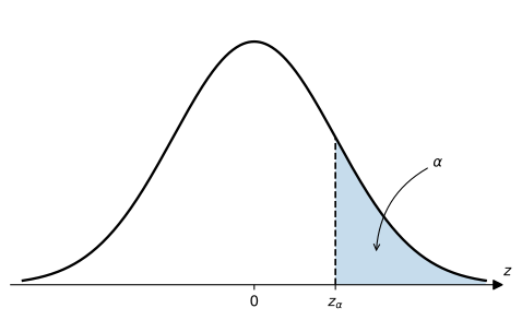
Like \operatorname{Φ}, its inverse has no closed form. In Python, norm.ppf computes it, so that z_{0.025} = \operatorname{Φ}^{-1}(0.975) is

print(norm.ppf(0.975))

1.959963984540054

In Excel, =norm.s.inv(0.975) gives the same result. The table below shows the values we use most often.

\boldsymbol{\alpha}	\boldsymbol{z_{\alpha}}
0.050	1.645
0.025	1.960
0.010	2.326
0.005	2.576

By symmetry, Z falls between -z_{\alpha/2} and z_{\alpha/2} with probability 1 - \alpha, leaving \alpha / 2 in each tail. For instance, Z lies in [-1.96, 1.96] with probability 95%.

Figure 6: The areas on each side are both equal to \alpha/2.

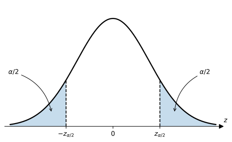
Since X = \mu + \sigma Z, the same statement for X \sim \mathcal{N}(\mu, \sigma^{2}) is that X lies in [\mu - z_{\alpha/2} \sigma, \mu + z_{\alpha/2} \sigma] with probability 1 - \alpha. We call this interval a (1 - \alpha) probability interval for X. It is often called a confidence interval, although in statistics that term refers to an interval estimated from data.

Example 4 Suppose that X \sim \mathcal{N}(\mu, \sigma^{2}) with \mu = 10 and \sigma = 25. Since z_{0.025} = 1.96, the 95% probability interval for X is [10 - 1.96 (25), 10 + 1.96 (25)] = [-39, 59].

Exponentials of a Normal Random Variable

One formula does most of the work in the rest of this chapter. It gives the expected value of e^{a X} for any constant a, the moment generating function of the normal distribution.

WarningExpected Exponential of a Normal Random Variable

If X \sim \mathcal{N}(\mu, \sigma^{2}), then for any constant a, \operatorname{E}\left(e^{a X}\right) = e^{a \mu + \frac{1}{2} a^{2} \sigma^{2}}. \tag{1}

Proof

Let \varphi(z) = e^{-z^{2}/2} / \sqrt{2 \pi} be the standard normal density. Completing the square, a z - \frac{1}{2} z^{2} = -\frac{1}{2} (z - a)^{2} + \frac{1}{2} a^{2}, so that e^{a z} \varphi(z) = e^{\frac{1}{2} a^{2}} \varphi(z - a). \tag{2} The right-hand side is e^{\frac{1}{2} a^{2}} times the density of a normal random variable with mean a and variance one, which integrates to one. Integrating both sides gives \operatorname{E}(e^{a Z}) = e^{\frac{1}{2} a^{2}} for a standard normal Z. Writing X = \mu + \sigma Z, \operatorname{E}\left(e^{a X}\right) = e^{a \mu} \operatorname{E}\left(e^{a \sigma Z}\right) = e^{a \mu + \frac{1}{2} a^{2} \sigma^{2}}.

The term \frac{1}{2} a^{2} \sigma^{2} in (1) is worth noticing. Since e^{x} is convex, the expected value of e^{a X} is larger than e^{a \operatorname{E}(X)} = e^{a \mu}, and the gap grows with the variance of X. The same term reappears in the next chapter as the difference between the expected return of a stock and the growth rate of its price.

The Lognormal Distribution

If X \sim \mathcal{N}(\mu, \sigma^{2}), then Y = e^{X} is lognormally distributed with parameters \mu and \sigma^{2}. The parameters are the mean and variance of \ln(Y), not of Y. Figure 7 compares the two densities.

Figure 7: The figure shows the difference between a normal and a lognormal PDF with the same parameters.

WarningLognormal Density

If Y is lognormally distributed with parameters \mu and \sigma^{2}, its PDF is f(y) = \frac{1}{y \sqrt{2 \pi \sigma^{2}}} e^{-\frac{(\ln(y) - \mu)^{2}}{2 \sigma^{2}}}, \qquad y > 0.

Proof

For y > 0, the CDF of Y is \operatorname{P}(Y \leq y) = \operatorname{P}(X \leq \ln(y)). Differentiating with respect to y and using the chain rule, the density of Y is the normal density of X evaluated at \ln(y), times the derivative d \ln(y) / dy = 1/y, which is the expression above.

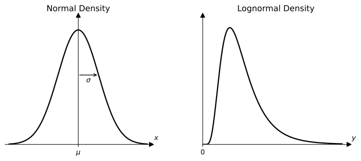
Unlike the normal density, the lognormal density is not symmetric. A normal random variable can take any real value, whereas a lognormal random variable is always positive, and its long right tail means that large values are more likely than equally distant small ones.

Computing Probabilities

The logarithm is an increasing function, so any statement about Y can be translated into a statement about the normal random variable \ln(Y): \operatorname{P}(Y \leq y) = \operatorname{P}(\ln(Y) \leq \ln(y)) = \operatorname{Φ}\left(\frac{\ln(y) - \mu}{\sigma}\right).

Example 5 Let Y = e^{4 + 1.5 Z} where Z \sim \mathcal{N}(0, 1). The probability that Y \leq 100 is \operatorname{P}(Y \leq 100) = \operatorname{P}\left(Z \leq \tfrac{\ln(100) - 4}{1.5}\right) = \operatorname{Φ}(0.4034) = 0.6567.

Probability intervals translate in the same way. If \ln(Y) lies in [\mu - z_{\alpha/2} \sigma, \mu + z_{\alpha/2} \sigma] with probability 1 - \alpha, then Y lies in [e^{\mu - z_{\alpha/2} \sigma}, e^{\mu + z_{\alpha/2} \sigma}] with the same probability.

Example 6 Let Y = e^{4 + 1.5 Z} where Z \sim \mathcal{N}(0, 1). The 95% probability interval for Y is [e^{4 - 1.96 (1.5)}, e^{4 + 1.96 (1.5)}] = [2.89, 1032.77]. The interval is far from symmetric around e^{4} = 54.60, the value of Y when \ln(Y) is at its mean.

Moments

Since Y^{a} = e^{a X}, the moments of Y follow directly from (1).

WarningMoments of a Lognormal Distribution

Let Y = e^{X} where X \sim \mathcal{N}(\mu, \sigma^{2}). For any constant a, \operatorname{E}(Y^{a}) = e^{a \mu + \frac{1}{2} a^{2} \sigma^{2}}. In particular, \begin{aligned} \operatorname{E}(Y) & = e^{\mu + \frac{1}{2} \sigma^{2}}, \\ \operatorname{V}(Y) & = e^{2\mu + \sigma^{2}} \left(e^{\sigma^{2}} - 1\right), \\ \operatorname{SD}(Y) & = \operatorname{E}(Y) \sqrt{e^{\sigma^{2}} - 1}. \end{aligned}

Proof

The first formula is (1). Taking a = 1 gives \operatorname{E}(Y), and taking a = 2 gives \operatorname{E}(Y^{2}) = e^{2 \mu + 2 \sigma^{2}}, so that \operatorname{V}(Y) = \operatorname{E}(Y^{2}) - \operatorname{E}(Y)^{2} = e^{2\mu + 2 \sigma^{2}} - e^{2\mu + \sigma^{2}} = e^{2\mu + \sigma^{2}} \left(e^{\sigma^{2}} - 1\right), and the standard deviation is its square root.

Example 7 Let Y = e^{4 + 1.5 Z} where Z \sim \mathcal{N}(0, 1). The expectation and standard deviation of Y are \begin{aligned} \operatorname{E}(Y) & = e^{4 + 0.5 (1.5^{2})} = 168.17, \\ \operatorname{SD}(Y) & = 168.17 \sqrt{e^{1.5^{2}} - 1} = 489.95. \end{aligned}

The mean of Y is not e^{\mu}. Half of the distribution of \ln(Y) lies below \mu, so the median of Y is e^{\mu}, while its mean e^{\mu + \frac{1}{2} \sigma^{2}} is larger. A few very large values pull the mean above the typical value. In Example 7 the median is e^{4} = 54.60 and the mean is 168.17, and Y falls below its mean with probability \operatorname{Φ}(\frac{1}{2} \sigma) = \operatorname{Φ}(0.75) = 0.7734.

Partial Expectations

A call option with strike price K pays Y - K if Y > K and nothing otherwise. To write such payoffs compactly, we use the indicator function 1\kern-0.25em\text{l}_{\{Y > K\}} = \begin{cases} 1 & \text{if $Y > K$,} \\ 0 & \text{if $Y \leq K$,} \end{cases} so that the payoff of the call is \max(Y - K, 0) = Y 1\kern-0.25em\text{l}_{\{Y > K\}} - K 1\kern-0.25em\text{l}_{\{Y > K\}}. Its expected value requires two partial expectations, which average Y and K only over the outcomes where the option is exercised.

WarningPartial Expectations

Let Y = e^{X} where X \sim \mathcal{N}(\mu, \sigma^{2}), let K > 0, and define d = \frac{\mu - \ln(K)}{\sigma}. Then \operatorname{P}(Y > K) = \operatorname{Φ}(d), \qquad \operatorname{E}\left(Y 1\kern-0.25em\text{l}_{\{Y > K\}}\right) = \operatorname{E}(Y) \operatorname{Φ}(d + \sigma), where \operatorname{E}(Y) = e^{\mu + \frac{1}{2} \sigma^{2}}. The second partial expectation is \operatorname{E}(K 1\kern-0.25em\text{l}_{\{Y > K\}}) = K \operatorname{P}(Y > K) = K \operatorname{Φ}(d).

Proof

Write Y = e^{\mu + \sigma Z} with Z standard normal. Then Y > K exactly when Z > -d, so that \operatorname{P}(Y > K) = 1 - \operatorname{Φ}(-d) = \operatorname{Φ}(d). For the partial expectation, (2) with a = \sigma gives \operatorname{E}\left(Y 1\kern-0.25em\text{l}_{\{Y > K\}}\right) = e^{\mu} \int_{-d}^{\infty} e^{\sigma z} \varphi(z) \, dz = e^{\mu + \frac{1}{2} \sigma^{2}} \int_{-d}^{\infty} \varphi(z - \sigma) \, dz = \operatorname{E}(Y) \operatorname{P}(Z + \sigma > -d), and \operatorname{P}(Z + \sigma > -d) = \operatorname{P}(Z > -(d + \sigma)) = \operatorname{Φ}(d + \sigma).

The first result is the probability that the option is exercised. The second is the full mean of Y times a probability whose argument is shifted from d to d + \sigma. Weighting each outcome by Y = e^{\mu + \sigma Z} gives more weight to high values of Z, and the effect is the same as shifting Z to the right by \sigma.

Example 8 Let Y = e^{4 + 1.5 Z} where Z \sim \mathcal{N}(0, 1), and let K = 100. Then d = (4 - \ln(100)) / 1.5 = -0.4034 and d + \sigma = 1.0966, so that \begin{aligned} \operatorname{P}(Y > 100) & = \operatorname{Φ}(-0.4034) = 0.3433, \\ \operatorname{E}\left(Y 1\kern-0.25em\text{l}_{\{Y > 100\}}\right) & = 168.17 \, \operatorname{Φ}(1.0966) = 145.23. \end{aligned} The expected payoff of a call on Y with strike price 100 is \operatorname{E}(\max(Y - 100, 0)) = 145.23 - 100 \times 0.3433 = 110.90.

The Black-Scholes chapter computes the price of a call in exactly this way: it takes the expected payoff of the option under a particular lognormal distribution and discounts it at the risk-free rate.

Practice Problems

Problem 1 Suppose that X is a normally distributed random variable with mean \mu=12 and standard deviation \sigma=20.

1. What is the probability that X \leq 0?
2. What is the probability that X \leq -4?
3. What is the probability that X > 8?
4. What is the probability that 4 < X \leq 10?

Solution

1. \operatorname{P}(X \leq 0) = \operatorname{Φ}(\frac{0-12}{20})
   \hphantom{\operatorname{P}(X \leq 0)} = \operatorname{Φ}(-0.60)
   \hphantom{\operatorname{P}(X \leq 0)} = 0.2743.

2. \operatorname{P}(X \leq -4) = \operatorname{Φ}(\frac{-4-12}{20})
   \hphantom{\operatorname{P}(X \leq -4)} = \operatorname{Φ}(-0.80)
   \hphantom{\operatorname{P}(X \leq -4)} = 0.2119.

3. \operatorname{P}(X > 8) = 1 - \operatorname{P}(X \leq 8)
   \hphantom{\operatorname{P}(X > 8)} = 1 - \operatorname{Φ}(\frac{8-12}{20})
   \hphantom{\operatorname{P}(X > 8)} = 1 - \operatorname{Φ}(-0.20)
   \hphantom{\operatorname{P}(X > 8)} = 0.5793.

4. \operatorname{P}(4 < X \leq 10) = \operatorname{P}(X \leq 10) - \operatorname{P}(X \leq 4)
   \hphantom{\operatorname{P}(4 < X \leq 10)} = \operatorname{Φ}(\frac{10-12}{20}) - \operatorname{Φ}(\frac{4-12}{20})
   \hphantom{\operatorname{P}(4 < X \leq 10)} = \operatorname{Φ}(-0.10) - \operatorname{Φ}(-0.40)
   \hphantom{\operatorname{P}(4 < X \leq 10)} = 0.1156.

Problem 2 Suppose that X is a normally distributed random variable with mean \mu=10 and standard deviation \sigma=20. Compute the 90%, 95%, and 99% probability intervals for X.

Solution

The (1-\alpha) probability interval for X is [\mu - z_{\alpha/2} \sigma, \mu + z_{\alpha/2} \sigma] where z_{\alpha/2} = \operatorname{Φ}^{-1}(1-\alpha/2). For the 90% interval, \alpha = 0.10 and \alpha/2 = 0.05, so z_{0.05} is =norm.s.inv(0.95) in Excel.

1. z_{0.05} = \operatorname{Φ}^{-1}(0.95) = 1.645, so the 90% interval for X is [-22.90, 42.90].
2. z_{0.025} = \operatorname{Φ}^{-1}(0.975) = 1.960, so the 95% interval for X is [-29.20, 49.20].
3. z_{0.005} = \operatorname{Φ}^{-1}(0.995) = 2.576, so the 99% interval for X is [-41.52, 61.52].

Problem 3 Suppose that X=\ln(Y) is a normally distributed random variable with mean \mu=3.9 and standard deviation \sigma=15.

1. What is the probability that Y \leq 6?
2. What is the probability that Y > 4?
3. What is the probability that 3 < Y \leq 12?
4. What is the probability that Y \leq 0?

Solution

1. \operatorname{P}(Y \leq 6) = \operatorname{P}(X \leq \ln(6))
   \hphantom{\operatorname{P}(Y \leq 6)} = \operatorname{Φ}(\frac{\ln(6)-3.9}{15})
   \hphantom{\operatorname{P}(Y \leq 6)} = \operatorname{Φ}(-0.1405)
   \hphantom{\operatorname{P}(Y \leq 6)} = 0.4441

2. \operatorname{P}(Y > 4) = 1 - \operatorname{P}(Y \leq 4)
   \hphantom{\operatorname{P}(Y > 4)} = 1 - \operatorname{P}(X \leq \ln(4))
   \hphantom{\operatorname{P}(Y > 4)} = 1 - \operatorname{Φ}(\frac{\ln(4)-3.9}{15})
   \hphantom{\operatorname{P}(Y > 4)} = 1 - \operatorname{Φ}(-0.1676)
   \hphantom{\operatorname{P}(Y > 4)} = 0.5665

3. \operatorname{P}(3 < Y \leq 12) = \operatorname{P}(Y \leq 12) - \operatorname{P}(Y \leq 3)
   \hphantom{\operatorname{P}(3 < Y \leq 12)} = \operatorname{Φ}(\frac{\ln(12)-3.9}{15}) - \operatorname{Φ}(\frac{\ln(3)-3.9}{15})
   \hphantom{\operatorname{P}(3 < Y \leq 12)} = \operatorname{Φ}(-0.0943) - \operatorname{Φ}(-0.1868)
   \hphantom{\operatorname{P}(3 < Y \leq 12)} = 0.4624 - 0.4259
   \hphantom{\operatorname{P}(3 < Y \leq 12)} = 0.0365

4. A lognormal random variable is always positive, so \operatorname{P}(Y \leq 0) = 0.

Problem 4 Suppose that X is a normally distributed variable with mean \mu=3.70 and standard deviation \sigma=0.80. If Y=e^{X}, what is the probability that Y is greater than 45?

Solution

\begin{aligned} \operatorname{P}(Y \leq 45) & = \operatorname{P}(\ln(Y) \leq \ln(45)) \\ & = \operatorname{P}\left( Z \leq \frac{\ln(45) - 3.70}{0.80} \right) \\ & = \operatorname{Φ}(0.1333) \\ & = 0.5530 \end{aligned} Therefore, \operatorname{P}(Y > 45) = 1 - 0.5530 = 0.4470.

Problem 5 Suppose that X=\ln(Y) is a normally distributed random variable with mean \mu=2.7 and standard deviation \sigma=1. Compute the 90%, 95%, and 99% probability intervals for X and report the corresponding values for Y.

Solution

The (1 - \alpha) probability interval for X is [\mu - z_{\alpha/2} \sigma, \mu + z_{\alpha/2} \sigma], and the corresponding interval for Y is [e^{\mu - z_{\alpha/2} \sigma}, e^{\mu + z_{\alpha/2} \sigma}].

1. z_{0.05} = 1.645, so the 90% interval for X is [1.06, 4.35], and the corresponding values for Y are [2.87, 77.09].
2. z_{0.025} = 1.960, so the 95% interval for X is [0.74, 4.66], and the corresponding values for Y are [2.10, 105.64].
3. z_{0.005} = 2.576, so the 99% interval for X is [0.12, 5.28], and the corresponding values for Y are [1.13, 195.59].

Problem 6 Let Y = e^{\mu + \sigma Z} where \mu = 1, \sigma = 2 and Z \sim \mathcal{N}(0, 1). Compute:

1. \operatorname{E}(Y)
2. \operatorname{SD}(Y) = \sqrt{\operatorname{E}(Y^{2}) - \operatorname{E}(Y)^{2}}
3. \operatorname{E}(Y^{0.3})
4. \operatorname{E}(Y^{-1})

Solution

All four answers use \operatorname{E}(Y^{a}) = e^{a\mu+\frac{1}{2}a^{2}\sigma^{2}}.

1. \operatorname{E}(Y) = e^{1+\frac{1}{2}2^{2}} = 20.09
2. \operatorname{E}(Y^{2}) = e^{(2)(1)+\frac{1}{2}(2)^{2}2^{2}}
   \hphantom{\operatorname{E}(Y^{2})} = 22026.47,
   \left(\operatorname{E}(Y)\right)^{2} = (20.09)^{2}
   \hphantom{\left(\operatorname{E}(Y)\right)^{2}} = 403.43,
   \operatorname{SD}(Y) = \sqrt{22026.47-403.43}
   \hphantom{\operatorname{SD}(Y)} = 147.05.
3. \operatorname{E}(Y^{0.3}) = e^{(0.3)(1)+\frac{1}{2}(0.3)^{2}2^{2}} = 1.62
4. \operatorname{E}(Y^{-1}) = e^{(-1)(1)+\frac{1}{2}(-1)^{2}2^{2}} = 2.72

Problem 7 Let Y = e^{X} where X \sim \mathcal{N}(\mu, \sigma^{2}) with \mu = 4.75 and \sigma = 0.35. Compute \operatorname{E}(Y 1\kern-0.25em\text{l}_{\{Y > 95\}}), \operatorname{P}(Y > 95), and the expected payoff \operatorname{E}(\max(Y - 95, 0)) of a call on Y with strike price 95.

Solution

The mean of Y is \operatorname{E}(Y) = e^{4.75 + 0.5 (0.35)^{2}} = 122.89, and d = (4.75 - \ln(95)) / 0.35 = 0.5604, so that d + \sigma = 0.9104. The partial expectations give \begin{aligned} \operatorname{P}(Y > 95) & = \operatorname{Φ}(0.5604) = 0.7124, \\ \operatorname{E}(Y 1\kern-0.25em\text{l}_{\{Y > 95\}}) & = 122.89 \, \operatorname{Φ}(0.9104) = 100.60, \end{aligned} so that \operatorname{E}(\max(Y - 95, 0)) = 100.60 - 95 \times 0.7124 = 32.92.