Modeling Stock Prices in Continuous-Time
The binomial model of Multiple Periods moves the stock price up by a factor u = e^{\sigma \sqrt{\Delta t}} or down by d = 1/u each period, and its prices approach the Black-Scholes prices as the periods get shorter. This chapter takes that limit. We describe the random part of the stock price with a Brownian motion, the continuous-time limit of a random walk, and model the stock price as a geometric Brownian motion. We then introduce Itô’s lemma, the chain rule for functions of a Brownian motion, which is the one tool from stochastic calculus that the Black-Scholes model needs. With it, we find the distribution of the future stock price, which is what the Black-Scholes formula needs.
The chapter assumes no background in stochastic processes, and it aims for intuition rather than proofs. The notes on Stochastic Foundations for Finance develop the same material with full arguments.
From Binomial Trees to Brownian Motion
The Log Price in a Binomial Tree
In a binomial tree with u = e^{\sigma \sqrt{\Delta t}} and d = e^{-\sigma \sqrt{\Delta t}}, each period adds \sigma \sqrt{\Delta t} to the logarithm of the stock price or subtracts it. After m periods, at time t = m \Delta t, \ln(S_{t}) = \ln(S_{0}) + \sigma \sqrt{\Delta t} \, (X_{1} + X_{2} + \cdots + X_{m}), where each X_{i} equals +1 for an up move and -1 for a down move. If up and down moves are equally likely and independent across periods, each X_{i} has mean zero and variance one, and \operatorname{V}\left(\ln(S_{t})\right) = \sigma^{2} \Delta t \times m = \sigma^{2} t. The variance of the log price grows in proportion to time, at the rate \sigma^{2}, however short the periods are. This is why the tree uses steps of size \sigma \sqrt{\Delta t}: with steps proportional to \Delta t, the variance would be \sigma^{2} t \Delta t and the stock price would stop moving as \Delta t \to 0, while with steps that do not shrink, the variance would explode.
The Scaled Random Walk
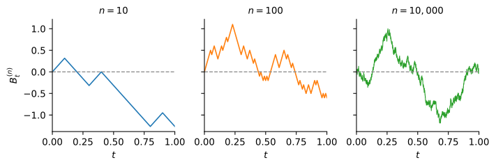
Setting \sigma aside, the random part of the log price is the scaled random walk B_{t}^{(n)} = \sqrt{\Delta t} \, (X_{1} + X_{2} + \cdots + X_{m}), \qquad t = m \Delta t, where n = 1 / \Delta t is the number of steps per unit of time. Its mean is zero and its variance is m \Delta t = t. Figure 1 shows one path of the walk for three values of n. With ten steps the path is a coarse zigzag. With ten thousand it looks like a continuous but very rough curve, and its range barely changes, since the variance at t = 1 is one for every n.
Brownian Motion
As \Delta t \to 0, the value of the walk at time t is a sum of more and more independent steps, each smaller than the last. By the central limit theorem, its distribution approaches a normal distribution with mean zero and variance t. The same is true of the change of the walk over any interval (s, t], which is built from the steps taken during that interval and is independent of the steps taken before. The limit of the scaled random walk is called a Brownian motion, or a Wiener process.
In particular, B_{t} \sim \mathcal{N}(0, t), so that B_{t} = \sqrt{t} \, Z for a standard normal Z. The increments are normal because of the central limit theorem, not because the coin flips were normal: any steps with mean zero and variance one would lead to the same limit.
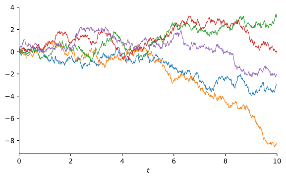
The paths in Figure 2 are continuous but nowhere smooth. Over a short interval of length dt, the increment dB has mean zero and standard deviation \sqrt{dt}, which is much larger than dt when dt is small. A Brownian path therefore moves a lot over every short interval, in one direction or the other. This single fact explains why calculus with Brownian motion differs from ordinary calculus, as we show below.
Geometric Brownian Motion
A Brownian motion is not a good model for the price itself. It can become negative, and its changes do not depend on its level, while a stock trading at $200 typically moves by about twice as many dollars in a day as the same stock trading at $100. What is roughly stable over time is the distribution of returns, the percentage changes in price. We therefore let returns, not price changes, be driven by a Brownian motion. Over a short interval of length \Delta t, the return on the stock is \frac{\Delta S_{t}}{S_{t}} = \mu \Delta t + \sigma \Delta B_{t}, which is normally distributed with mean \mu \Delta t and variance \sigma^{2} \Delta t. Letting \Delta t \to 0 gives dS = \mu S \, dt + \sigma S \, dB. \tag{1} The process \{S_{t}\} is called a geometric Brownian motion (GBM). The constant \mu is the expected return of the stock per unit of time, and \sigma is the volatility of its returns, the same \sigma used to build binomial trees. Both are usually quoted per year. Equation (1) is shorthand for the limit of the discrete returns above, and it says that over each short interval the stock earns a deterministic return \mu \, dt plus a random return \sigma \, dB.
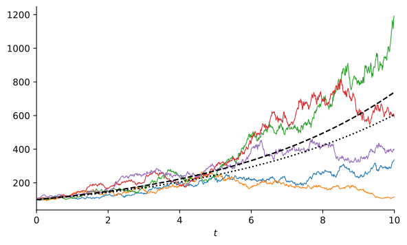
Figure 3 shows that the paths never fall below zero, that their fluctuations grow with the price level, and that they fan out unevenly, with a few ending far above the rest. To make these statements precise, we need the distribution of S_{T}, and to find it we need a rule for how functions of S_{t}, such as \ln(S_{t}), change over time.
Itô’s Lemma
Why Ordinary Calculus Fails
In ordinary calculus, if x changes by a small amount \Delta x, a smooth function F(x) changes by \Delta F \approx F'(x) \, \Delta x + \frac{1}{2} F''(x) (\Delta x)^{2}, and the second-order term is negligible because (\Delta x)^{2} is tiny compared with \Delta x. For a Brownian motion, \Delta B is of order \sqrt{\Delta t}, so (\Delta B)^{2} is of order \Delta t, the same order as the time step itself. The second-order term no longer disappears.
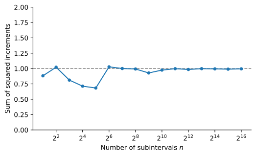
More precisely, (\Delta B)^{2} = \Delta t \, Z^{2} for a standard normal Z, so it has mean \Delta t and variance 2 (\Delta t)^{2}. Its standard deviation, \sqrt{2} \, \Delta t, is as large as its mean, so a single squared increment is far from \Delta t. But split an interval [0, t] into n steps of length \Delta t = t/n and add up the squared increments of a Brownian path. The squared increments are independent, so their sum has mean n \Delta t = t and variance n \times 2 (\Delta t)^{2} = 2 t \, \Delta t, which goes to zero as \Delta t \to 0. The sum of squared increments converges to t, on every path. Figure 4 shows this for one simulated path on [0, 1].
In differential notation, this result reads (dB)^{2} = dt. The squared increments of a Brownian motion add up like increments of time, so in any calculation that adds up many small changes, (dB)^{2} can be replaced by dt. The products (dt)^{2} and (dt)(dB) are of order (dt)^{2} and (dt)^{3/2}, smaller than dt, and they add up to zero. Together, these rules are called the multiplication table or box calculus.
For a GBM, the multiplication table gives (dS)^{2} = (\mu S \, dt + \sigma S \, dB)^{2} = \mu^{2} S^{2} (dt)^{2} + 2 \mu \sigma S^{2} (dt)(dB) + \sigma^{2} S^{2} (dB)^{2} = \sigma^{2} S^{2} \, dt. The drift does not contribute to (dS)^{2}. Only the random term, which moves the price by amounts of order \sqrt{dt}, does.
The Lemma
Expanding a function F(S, t) to second order in dS and first order in dt, and keeping the term (dS)^{2} = \sigma^{2} S^{2} \, dt that ordinary calculus would drop, gives Itô’s lemma.
Sketch of proof
A second-order Taylor expansion of F gives dF = \frac{\partial F}{\partial S} dS + \frac{\partial F}{\partial t} dt + \frac{1}{2} \frac{\partial^{2} F}{\partial S^{2}} (dS)^{2} + \frac{\partial^{2} F}{\partial S \partial t} (dS)(dt) + \frac{1}{2} \frac{\partial^{2} F}{\partial t^{2}} (dt)^{2}. By the multiplication table, (dS)^{2} = \sigma^{2} S^{2} dt, while (dS)(dt) = \mu S (dt)^{2} + \sigma S (dB)(dt) = 0 and (dt)^{2} = 0. Higher-order terms involve (dS)^{3} and higher powers, which are of order (dt)^{3/2} or smaller and also vanish. What is left is Itô’s lemma.The term \frac{1}{2} \sigma^{2} S^{2} \frac{\partial^{2} F}{\partial S^{2}} is the Itô correction. It has no counterpart in ordinary calculus, and it vanishes when there is no randomness (\sigma = 0) or when F is linear in S. When F depends only on S, the last term drops out. Equation (2) also shows that F is driven by the same Brownian motion as the stock, with a random term \sigma S \frac{\partial F}{\partial S} dB that is proportional to the sensitivity of F to the stock price. This common source of risk is what allows an option to be replicated with the stock in the Black-Scholes model.
Example 1 Let F(S, t) = e^{-r t} S be the stock price discounted at the risk-free rate r. Then \frac{\partial F}{\partial S} = e^{-r t}, \frac{\partial^{2} F}{\partial S^{2}} = 0, and \frac{\partial F}{\partial t} = -r e^{-r t} S, so that dF = \left(\mu e^{-r t} S - r e^{-r t} S\right) dt + \sigma e^{-r t} S \, dB = (\mu - r) F \, dt + \sigma F \, dB. The discounted stock price is again a GBM, with expected return \mu - r, the risk premium of the stock, and the same volatility. There is no Itô correction because F is linear in S.
Solving for the Stock Price
The logarithm turns multiplicative changes into additive ones, so we apply Itô’s lemma to F(S) = \ln(S). With \frac{\partial F}{\partial S} = 1/S and \frac{\partial^{2} F}{\partial S^{2}} = -1/S^{2}, \begin{aligned} d\ln(S) & = \frac{1}{S} \, dS + \frac{1}{2} \left(-\frac{1}{S^{2}}\right) (dS)^{2} \\ & = \frac{1}{S} \left(\mu S \, dt + \sigma S \, dB\right) - \frac{1}{2} \frac{1}{S^{2}} \sigma^{2} S^{2} \, dt \\ & = \left(\mu - \tfrac{1}{2} \sigma^{2}\right) dt + \sigma \, dB. \end{aligned} The right-hand side has constant coefficients, so the changes of \ln(S) add up to \ln(S_{T}) - \ln(S_{0}) = \left(\mu - \tfrac{1}{2} \sigma^{2}\right) T + \sigma B_{T}, and taking exponentials, S_{T} = S_{0} \exp\left(\left(\mu - \tfrac{1}{2} \sigma^{2}\right) T + \sigma B_{T}\right). \tag{3}
The log price is a Brownian motion with drift \mu - \frac{1}{2} \sigma^{2} and volatility \sigma, the continuous-time version of the log price in a binomial tree. The term -\frac{1}{2} \sigma^{2} is the Itô correction. Ordinary calculus would give d\ln(S) = dS/S, and a log price that grows at the rate \mu.
The Distribution of the Stock Price
Since B_{T} \sim \mathcal{N}(0, T), equation (3) implies that the log price is normally distributed, \ln(S_{T}) \sim \mathcal{N}(m, s^{2}), \qquad m = \ln(S_{0}) + \left(\mu - \tfrac{1}{2} \sigma^{2}\right) T, \qquad s = \sigma \sqrt{T}. In other words, S_{T} has a lognormal distribution, as defined in The Lognormal Distribution. The continuously compounded return \ln(S_{T} / S_{0}) over a horizon T is normal, with mean \left(\mu - \frac{1}{2} \sigma^{2}\right) T and standard deviation \sigma \sqrt{T}. Probabilities about the stock price are computed by translating them into statements about this normal return.
Example 2 A stock that follows a GBM has an expected return of 12% per year and a volatility of 25% per year, and its current price is $25. Over T = 0.5 years, the log price X_{T} = \ln(S_{T}) has \begin{aligned} \operatorname{E}(X_{T}) & = \ln(25) + \left(0.12 - 0.5 (0.25)^{2}\right)(0.5) = 3.2633, \\ \operatorname{SD}(X_{T}) & = 0.25 \sqrt{0.5} = 0.1768. \end{aligned} The 95% probability interval for X_{T} is 3.2633 \pm 1.96 (0.1768), and exponentiating its endpoints gives \left[e^{3.2633 - 1.96 (0.1768)}, e^{3.2633 + 1.96 (0.1768)}\right] = [18.48, 36.96]. There is a 95% probability that the stock price in six months will lie between $18.48 and $36.96. The interval is not symmetric around the current price, because the lognormal distribution is skewed to the right.
Moments of the Stock Price
The moments of a lognormal random variable from The Lognormal Distribution give the mean and standard deviation of S_{T}.
Proof
Since \ln(S_{T}) \sim \mathcal{N}(m, s^{2}), \operatorname{E}(S_{T}) = e^{m + \frac{1}{2} s^{2}} = e^{\ln(S_{0}) + \left(\mu - \frac{1}{2} \sigma^{2}\right) T + \frac{1}{2} \sigma^{2} T} = S_{0} e^{\mu T}, and \operatorname{SD}(S_{T}) = \operatorname{E}(S_{T}) \sqrt{e^{s^{2}} - 1} with s^{2} = \sigma^{2} T.The expected stock price grows at the rate \mu, which is why \mu is called the expected return. The standard deviation is proportional to the expected price and grows even faster, so the uncertainty about the future price grows much faster than the expected price.
Example 3 For the stock in Example 2, the expected price and the standard deviation of the price six months from now are \begin{aligned} \operatorname{E}(S_{T}) & = 25 e^{0.12 (0.5)} = \$26.55, \\ \operatorname{SD}(S_{T}) & = 26.55 \sqrt{e^{0.25^{2} (0.5)} - 1} = \$4.73. \end{aligned}
Expected Return and Growth Rate
The log price grows at the rate \mu - \frac{1}{2} \sigma^{2}, while the expected price grows at the faster rate \mu. Both statements are correct, and the gap between them comes from the skewness of the lognormal distribution. The median of S_{T} is the price at which the log price is at its mean, \text{Median}(S_{T}) = S_{0} e^{\left(\mu - \frac{1}{2} \sigma^{2}\right) T} < S_{0} e^{\mu T} = \operatorname{E}(S_{T}). Half of the paths end below the median, and more than half end below the mean. A few paths that end very high pull the mean above what a typical path achieves, as the dashed and dotted lines in Figure 3 show. The rate \mu - \frac{1}{2} \sigma^{2} is the growth rate that an investor holding the stock for a long time will typically realize, while \mu is the rate at which wealth grows on average across all paths.
Example 4 A stock has an expected return of \mu = 0.10 and a volatility of \sigma = 0.20. Its log price grows at the rate 0.10 - 0.5 (0.20)^{2} = 0.08 per year. Over T = 10 years, the expected price is e^{0.10 \times 10} = 2.72 times the current price, but the median price is only e^{0.08 \times 10} = 2.23 times the current price. The stock ends below its expected price when \sigma B_{T} < \frac{1}{2} \sigma^{2} T, which has probability \operatorname{P}\left(Z < \tfrac{1}{2} \sigma \sqrt{T}\right) = \operatorname{Φ}(0.3162) = 0.6241, where Z is a standard normal random variable.
The Black-Scholes model prices options with this lognormal distribution, with one change: the expected return \mu is replaced by the risk-free rate r. The Black-Scholes Model explains why.
Practice Problems
Problem 1 Consider a stock whose price at time t is given by S_{t} and that follows a geometric Brownian motion (GBM). The expected return is 18% per year and the volatility is 32% per year. The current spot price is $60.
- Compute the expected price 9 months from now.
- Compute the mean and standard deviation of the log-spot price 9 months from now.
- Compute the 95% probability interval of \ln(S_{T}) 9 months from now, and report the corresponding values for S_{T}.
Solution
- \operatorname{E}(S_{T}) = 60 e^{0.18(9/12)} = \$68.67.
- The mean and standard deviation can be computed as follows: \begin{aligned} m & = \ln(60) + (0.18 - 0.5(0.32^{2}))(9/12) \\ & = 4.1909 \\ s & = 0.32 \sqrt{9/12} \\ & = 0.2771 \end{aligned}
- The probability interval of \ln(S_{T}) 9 months from now satisfies: \begin{aligned} \operatorname{P}\left( -1.96 < \frac{\ln(S_{T}) - m}{s} \leq 1.96 \right) & = \operatorname{P}\left(m - 1.96 s < \ln(S_{T}) \leq m + 1.96 s \right) \\ & = \operatorname{P}(3.6478 < \ln(S_{T}) \leq 4.7341) \\ & = \operatorname{P}\left(e^{3.6478} < S_{T} \leq e^{4.7341}\right) \\ & = \operatorname{P}(38.39 < S_{T} \leq 113.76) \end{aligned} Therefore, the 95% probability interval for \ln(S_{T}) is [3.6478, 4.7341] and the corresponding values for S_{T} are [38.39, 113.76].
Problem 2 Consider a stock whose price at time t is given by S_{t} and that follows a GBM. The expected return is 11% per year and the volatility is 27% per year. The current spot price is $60.
- Compute the expected price of S_{t} 1 year from now.
- Compute the expected price of 1 / S_{t} 1 year from now.
Solution
- \operatorname{E}(S_{T}) = 60 e^{0.11(1)} = \$66.98
- We have that \ln(S_{T}) \sim \mathcal{N}(m, s^{2}), where: \begin{aligned} m & = \ln(60) + (0.11 - 0.5(0.27^{2}))(1) \\ & = 4.1679 \\ s & = 0.27 \sqrt{1} \\ & = 0.27 \end{aligned} Using \operatorname{E}(Y^{a}) = e^{a m + \frac{1}{2} a^{2} s^{2}} for Y = S_{T} and a = -1, \begin{aligned} \operatorname{E}(1/S_{T}) & = e^{(-1)4.1679 + 0.5(-1)^{2}(0.27)^{2}} \\ & = 0.0161 \end{aligned}
Problem 3 Consider a stock whose price at time t is given by S_{t} and that follows a GBM. The expected return is 12% per year and the volatility is 35% per year. The current spot price is $55. Let T=18 months.
- Compute \operatorname{E}(S_{T}).
- Compute the mean and standard deviation of the log-spot price at T.
- Find C such that \operatorname{P}(S_{T} \leq C)=0.01.
Solution
- \operatorname{E}(S_{T}) = 55 e^{0.12(18/12)} = \$65.85
- We have that \ln(S_{T}) \sim \mathcal{N}(m, s^{2}), where: \begin{aligned} m & = \ln(55) + (0.12 - 0.5(0.35^{2}))(18/12) \\ & = 4.0955 \\ s & = 0.35 \sqrt{18/12} \\ & = 0.4287 \end{aligned}
- We want to find C such that: \begin{aligned} \operatorname{P}(S_{T} \leq C) & = \operatorname{P}\left(Z \leq \tfrac{\ln(C) - m}{s}\right) \\ & = 0.01 \end{aligned} Hence, \dfrac{\ln(C) - 4.0955}{0.4287} = -2.326, which implies that: \begin{aligned} \ln(C) & = 4.0955 - 2.326(0.4287) \\ & = 3.0982 \end{aligned} Therefore, C = e^{3.0982} = \$22.16.
Problem 4 Consider a stock whose price at time T is given by S_{T} and that follows a GBM, i.e., \ln(S_{T}) \sim \mathcal{N}(\ln(S_{0})+(\mu-0.5\sigma^{2})T, \sigma^{2} T).
The expected return is 12% per year and the volatility is 35% per year. The current spot price is $100.
- Compute the expected price in 2 years from now.
- Compute the mean and standard deviation of the log-spot price in 2 years from now.
- Compute the probability that the spot price is less than $100 in 2 years from now.
- Compute the probability that the spot price is greater than $120 in 2 years from now.
Solution
- \operatorname{E}(S_{T}) = 100 e^{0.12(2)} = \$127.12
- We have that \ln(S_{T}) \sim \mathcal{N}(m, s^{2}), where: \begin{aligned} m & = \ln(100) + (0.12 - 0.5(0.35^{2}))(2) = 4.7227 \\ s & = 0.35 \sqrt{2} = 0.4950 \end{aligned}
- The probability that S_{T} \leq 100 is: \begin{aligned} \operatorname{P}(S_{T} \leq 100) & = \operatorname{P}(\ln(S_{T}) \leq \ln(100)) \\ & = \operatorname{P}\left(Z \leq \frac{\ln(100) - 4.7227}{0.4950}\right) \\ & = \operatorname{Φ}(-0.2374) \\ & = 0.4062 \end{aligned}
- The probability that S_{T} > 120 is: \begin{aligned} \operatorname{P}(S_{T} > 120) & = 1 - \operatorname{P}(S_{T} \leq 120) \\ \operatorname{P}(S_{T} \leq 120) & = \operatorname{P}(\ln(S_{T}) \leq \ln(120)) \\ & = \operatorname{P}\left(Z \leq \frac{\ln(120) - 4.7227}{0.4950}\right) \\ & = \operatorname{Φ}(0.1310) \\ & = 0.5521 \end{aligned} Hence, \operatorname{P}(S_{T} > 120) = 1 - 0.5521 = 0.4479.
Problem 5 Suppose that the stock price follows a geometric Brownian motion (GBM) with drift \mu and instantaneous volatility \sigma, i.e., dS = \mu S dt + \sigma S dB. Show that Y = S^{\alpha} also follows a GBM and determine the drift and volatility as a function of \mu, \sigma, and \alpha.
Solution
We have that Y'(S) = \alpha S^{\alpha - 1} and Y''(S) = \alpha (\alpha - 1) S^{\alpha - 2}. Therefore, \begin{aligned} dY & = Y'(S)\, (dS) + \frac{1}{2} Y''(S)\, (dS)^{2} \\ & =\alpha S^{\alpha - 1} (\mu S dt + \sigma S dB) + \frac{1}{2} \alpha (\alpha - 1) S^{\alpha - 2} (\sigma^{2} S^{2} dt) \\ & = \left(\alpha \mu S^{\alpha} + \frac{1}{2} \alpha (\alpha - 1) \sigma^{2} S^{\alpha}\right) dt + \alpha \sigma S^{\alpha} dB \\ & = \left(\alpha \mu + \frac{1}{2} \alpha (\alpha - 1) \sigma^{2} \right) Y dt + \alpha \sigma Y dB \\ \end{aligned} Hence, Y follows a GBM with drift \alpha \mu + \frac{1}{2} \alpha (\alpha - 1) \sigma^{2} and volatility \alpha \sigma.Problem 6 Let S be the price of TESLA stock that follows a geometric Brownian motion such that dS = \mu S dt + \sigma S dB. Your sales team would like to launch a new product called TESLA Quadro that tracks the price of TESLA to the power 4. In other words, the value of this instrument is given by Y = S^{4}. What is the process followed by Y?
Solution
By Itô’s lemma, dY = Y'(S)\, dS + \frac{1}{2} Y''(S)\, (dS)^{2}, where (dS)^{2} = \sigma^{2} S^{2} dt. If Y = S^{4} then Y'(S) = 4 S^{3} and Y''(S) = 12 S^{2}. We can then write the previous expression as \begin{aligned} dY & = 4 S^{3} (\mu S dt + \sigma S dB) + \frac{1}{2} (12 S^{2}) (\sigma^{2} S^{2} dt) \\ & = 4 \mu S^{4} dt + 4 \sigma S^{4} dB + 6 \sigma^{2} S^{4} dt \\ & = (4 \mu + 6 \sigma^{2}) Y dt + 4 \sigma Y dB \end{aligned} The new product then follows a geometric Brownian motion with drift 4 \mu + 6 \sigma^{2} and instantaneous volatility 4 \sigma.Problem 7 GoingUp Corp. has been gaining a lot of attention in the media for its upside potential. Financial experts agree that the stock price follows a geometric Brownian motion with drift (\mu) equal to 20% per year and volatility of price returns (\sigma) of 73% per year. The current stock price is $220. Compute the probability that the stock price is greater than $233 in 10 months from now.
Solution
We know that \ln(S_{T}) \sim \mathcal{N}(m, s^{2}) where \begin{aligned} m & = \ln(S_{0}) + (\mu - 0.5 \sigma^{2}) T \\ & = \ln(220) + (0.20 - 0.5 \times 0.73^{2}) \times (10/12) \\ & = 5.3383 \\ s & = \sigma \sqrt{T} \\ & = 0.73 \sqrt{10/12} \\ & = 0.6664 \end{aligned} Therefore, \begin{aligned} \operatorname{P}(S_{T} \leq 233) & = \operatorname{P}(\ln(S_{T}) \leq \ln(233)) \\ & = \operatorname{P}\left( Z \leq \frac{\ln(233) - 5.3383}{0.6664} \right) \\ & = \operatorname{Φ}(0.1692) \\ & = 0.5672 \end{aligned} Therefore, \operatorname{P}(S_{T} > 233) = 1 - 0.5672 = 0.4328.Problem 8 You would like to invest in ZigZag Inc. but you are concerned that the stock price might go down. You have been studying the dynamics of the stock price and concluded that the stock follows a geometric Brownian motion with drift (\mu) equal to 13% per year and volatility of price returns (\sigma) of 58% per year. The current stock price is $118. Compute the probability that the stock price is less than $98 in 12 months from now.
Solution
We know that \ln(S_{T}) \sim \mathcal{N}(m, s^{2}) where \begin{aligned} m & = \ln(S_{0}) + (\mu - 0.5 \sigma^{2}) T \\ & = \ln(118) + (0.13 - 0.5 \times 0.58^{2}) \\ & = 4.7325 \\ s & = \sigma \sqrt{T} \\ & = 0.58 \end{aligned} Therefore, \begin{aligned} \operatorname{P}(S_{T} \leq 98) & = \operatorname{P}(\ln(S_{T}) \leq \ln(98)) \\ & = \operatorname{P}\left( Z \leq \frac{\ln(98) - 4.7325}{0.58} \right) \\ & = \operatorname{Φ}(-0.2543) \\ & = 0.3996 \end{aligned}Problem 9 You are analyzing BMX stock. You believe that it is accurate to model the price evolution of the stock as a geometric Brownian motion. Using historical data, you estimate that the drift (\mu) is 12.0% per year and the volatility of stock returns (\sigma) is 39% per year. The stock price just closed at $331. Compute the expected stock price in 9 months from now.