Options on Assets Paying a Dividend Yield
General Framework
The Dividend Yield
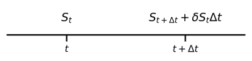
We introduced the continuously-compounded dividend yield \delta in The Impact of Dividends, where it changed put-call parity and the option bounds. Here we make the timing of the payment precise. Over each short interval \Delta t, the asset S pays a dividend of \delta \Delta t shares and therefore \delta S_{t} \Delta t dollars. Therefore, if you purchase one unit of the asset at time t for S_{t}, the value of the portfolio at time t + \Delta t will be S_{t + \Delta t} + \delta S_{t} \Delta t.
You will notice that the payment of the dividend at time t + \Delta t is known at time t. Indeed, this payment depends on the value of the stock at time t and not t + \Delta t. This is not a mistake or a convenience, but reflects the fact that we want to incorporate in the total return of investing in the stock from time t to t + \Delta t both capital gains and dividends: \underbrace{\frac{S_{t + \Delta t} + \delta S_{t} \Delta t - S_{t}}{S_{t}}}_{\text{Total Return}} = \underbrace{\frac{\Delta S_{t}}{S_{t}}}_{\text{Capital Gains}} + \underbrace{\vphantom{\frac{\Delta S_{t}}{S_{t}}} \delta \Delta t}_{\text{Dividends}}. \tag{1} In practice, this is the approach used to model options on stock indices and foreign currencies, although some practitioners also use it to model individual stocks as well. We must note that especially for American type options, modelling lump-sum dividends as a continuous yield might induce errors in computing the optimal early-exercise policy. It could also lead to the wrong risk-neutral adjustment if dividends are paid, say, twice per year, and we want to risk-adjust the underlying asset process for the next three months just after a dividend has been paid.
Replicating A Derivative
As we did in the previous chapter where there were no dividends, to price a call or put option we take the point of view of a trading desk that makes the market for such contracts. Their sales team just sold a European option H written on a stock S with maturity T to a client. The stock in this case, though, pays a continuous dividend yield \delta.
The traders of the desk will replicate the option by buying (or selling) N_{S} units of the stock and N_{Z} units of a bond with face value K and maturity T, respectively. The difference in this case compared to the no-dividend stock is that the number of shares bought will grow, so that the trader will have to buy a little less in order to hedge a call option, for example.
If we call V the value of such replicating portfolio, we have that: V_{t} = N_{S, t} S_{t} + N_{Z, t} Z_{t}. \tag{2} At time t+\Delta t, and because the underlying asset pays dividends, the value of the replicating portfolio is: V_{t + \Delta t} = N_{S, t} (S_{t + \Delta t} + \delta S_{t} \Delta t) + N_{Z, t} Z_{t + \Delta t}, which implies that: \Delta V_{t} = N_{S, t} (\Delta S_{t} + \delta S_{t} \Delta t) + N_{Z, t} \Delta Z_{t}.
As \Delta t \rightarrow 0, we have that: \begin{aligned} dV & = N_{S} (dS + \delta S dt) + N_{Z} dZ \\ & = N_{S} (dS + \delta S dt) + (N_{Z} Z) r dt \\ & = N_{S} (dS + \delta S dt) + r (V - N_{S} S) dt \\ & = \left(r V - (r - \delta) N_{S} S\right) dt + N_{S} dS, \end{aligned} \tag{3} where in the second line we used the fact that dZ = r Z dt, and in the third line we applied the self-financing condition (2) re-written as N_{Z} Z = V - N_{S} S.
As in the previous chapter, equation (3) captures the dynamics of the replicating portfolio needed to hedge the short position. For the hedge to be successful, the dynamics of the long position must match the dynamics of the short position that are given by: dV = \frac{\partial V}{\partial S} dS + \frac{1}{2} \sigma^{2} S^{2} \frac{\partial^{2} V}{\partial S^{2}} dt + \frac{\partial V}{\partial t} dt. \tag{4} Equating (3) and (4) shows that: \left(\frac{1}{2} \sigma^{2} S^{2} \frac{\partial^{2} V}{\partial S^{2}} + \frac{\partial V}{\partial t}\right) dt + \frac{\partial V}{\partial S} dS = \left(r V - (r - \delta) N_{S} S\right) dt + N_{S} dS. \tag{5} Equation (5) reveals that, even in the presence of a dividend yield, the number of shares required to hedge the option must equal the partial derivative with respect to the stock price. Therefore, choosing N_{S} = \frac{\partial V}{\partial S} implies that: \frac{1}{2} \sigma^{2} S^{2} \frac{\partial^{2} V}{\partial S^{2}} + (r - \delta) S \frac{\partial V}{\partial S} + \frac{\partial V}{\partial t} - r V = 0 \tag{6} with boundary condition V_{T} = F(S_{T}).
Equation (6) is the Black-Scholes partial differential equation (PDE) that must satisfy all derivatives written on an asset that pays a dividend yield.1
1 The Black-Scholes PDE given by (6) is only valid for derivative instruments (or assets) that do not pay dividends themselves, even though they are written on a dividend paying asset. The stock, for example, does not satisfy equation (6) since it pays a dividend. A generalized PDE that allows for the derivative to also pay a dividend yield can be found in the appendix.
Example 1 Consider a forward contract written on an asset that pays a dividend yield \delta expiring at time T with forward price K. The value V of the forward contract at time 0 \leq t \leq T is: V = S e^{-\delta (T - t)} - K e^{-r (T - t)} Let us check that the value of the contract satisfies the Black-Scholes PDE equation (6). The relevant derivatives are \begin{aligned} \frac{\partial V}{\partial S} & = e^{-\delta (T - t)}, \\ \frac{\partial^{2} V}{\partial S^{2}} & = 0, \\ \frac{\partial V}{\partial t} & = \delta S e^{-\delta(T - t)} - r K e^{-r (T - t)}. \\ \end{aligned} The left-hand side of equation (6) then becomes (r - \delta) S e^{-\delta (T - t)} + \delta S e^{-\delta (T - t)} - r K e^{-r (T - t)} - r (S e^{-\delta (T - t)} - K e^{-r (T - t)}) = 0, which clearly satisfy the claim.
The Risk-Neutral Process for the Underlying Asset
As in the Black-Scholes model, the replication argument is indifferent of the dynamics of the stock. This implies that the same logic should work in a hypothetical world where everyone is risk-neutral. In such a world, the expected total return of all assets is the risk-free rate. Hence, equation (1) implies that: \frac{S_{t + \Delta t} + \delta S_{t} \Delta t - S_{t}}{S_{t}} = \frac{\Delta S_{t}}{S_{t}} + \delta \Delta t = r \Delta t + \sigma \Delta B^{*}_{t}. As \Delta t \rightarrow 0 we obtain the continuous-time analog of risk-neutral process followed by the stock: dS = (r - \delta) S dt + \sigma S dB^{*}. We conclude that S follows a GBM under the risk-neutral measure with drift r - \delta and volatility \sigma.
Example 2 We can use the risk-neutral approach to compute the value V of a long forward contract with maturity T and forward price K. The payoff of the long forward at maturity is given by S_{T} - K.
The value of the contract is then the expected payoff discounted at the risk-free rate, i.e., \begin{aligned} V & = e^{-r T} \operatorname{E}^{*}(S_{T} - K) \\ & = e^{-r T} (S e^{(r - \delta) T} - K) \\ & = S e^{-\delta T} - K e^{-r T}. \end{aligned} The value of the forward, in general, will change over time. The forward price F is determined such that the value of the contract is zero when the contract is signed. Thus, V = S e^{-\delta T} - F e^{-r T} = 0 \Rightarrow F = S e^{(r - \delta) T}.
Remember that under the risk-neutral measure, the value of any asset is computed as its expected payoff discounted at the risk-free rate. Therefore, the price of a European call option with maturity T and strike price K written on the asset that pays a continuous dividend yield \delta is given by: \begin{aligned} C & = e^{-r T} \operatorname{E}^{*}\left((S_{T} - K) 1\kern-0.25em\text{l}_{\{S_{T} > K\}} \right) \\ & = e^{-r T} \operatorname{E}^{*}\left(S_{T} 1\kern-0.25em\text{l}_{\{S_{T} > K\}} \right) - e^{-r T} \operatorname{E}^{*}\left(K 1\kern-0.25em\text{l}_{\{S_{T} > K\}} \right) \\ & = S e^{-\delta T} \operatorname{Φ}(d_{1}) - K e^{-r T} \operatorname{Φ}(d_{2}), \end{aligned} where \begin{aligned} d_{1} & = \frac{\ln(S/K) + (r - \delta + \frac{1}{2} \sigma^{2}) T}{\sigma \sqrt{T}}, \\ d_{2} & = d_{1} - \sigma \sqrt{T}. \end{aligned}
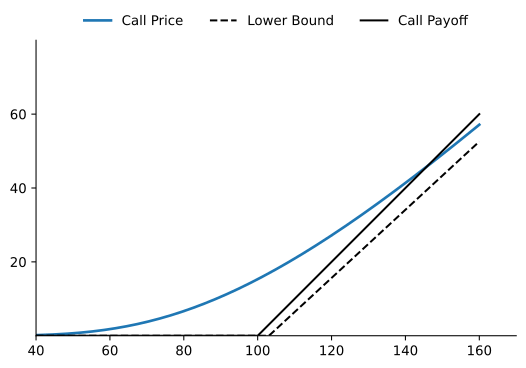
Note that, even though the risk-free rate is positive, the time-value of deep ITM call options is now negative due to the positive dividend yield. Indeed, the lower bound asymptote has a slope coefficient less than one, making the option price to cross the option’s intrinsic value.
Consider now a European put option with the same characteristics as the previous call. According to put-call parity, it must be the case that C - P = S e^{-\delta T} - K e^{-r T}. Hence, \begin{aligned} P & = C - (S e^{-\delta T} - K e^{-rT}) \\ & = S e^{-\delta T} \operatorname{Φ}(d_{1}) - K e^{-r T} \operatorname{Φ}(d_{2}) - (S e^{-\delta T} - K e^{-rT}) \\ & = K e^{-r T} (1 - \operatorname{Φ}(d_{2})) - S e^{-\delta T} (1 - \operatorname{Φ}(d_{1})) \\ & = K e^{-r T} \operatorname{Φ}(-d_{2}) - S e^{-\delta T} \operatorname{Φ}(-d_{1}). \end{aligned}
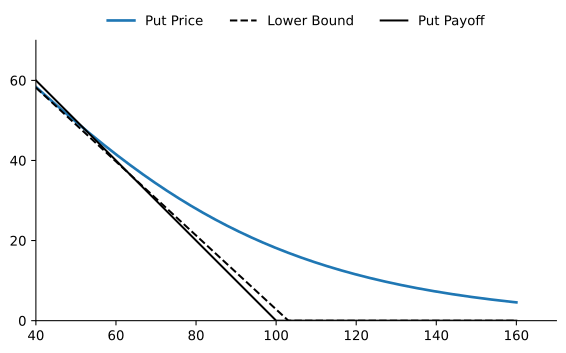
Example 3 A stock that pays a continuous dividend yield of 8% currently trades for $100. The instantaneous volatility of returns is 30% per year and the risk-free rate is 5% per year, continuously compounded and constant for all maturities. Consider ATM call and put options written on the stock with maturity 10 months. Then, \begin{aligned} d_{1} & = \frac{\ln(100/100) + (0.05 - 0.08 + 0.5(0.30)^{2})(10/12)}{0.30\sqrt{10/12}} = 0.0456, \\ d_{2} & = 0.0456 - 0.30\sqrt{10/12} = -0.2282. \end{aligned} Therefore, \operatorname{Φ}(d_{1}) = 0.5182 and \operatorname{Φ}(d_{2}) = 0.4097, which implies that \begin{aligned} C & = 100e^{-0.08(10/12)}(0.5182) - 100e^{-0.05(10/12)}(0.4097) = \$9.18, \\ P & = 100e^{-0.05(10/12)}(1 - 0.4097) - 100e^{-0.08(10/12)}(1 - 0.5182) = \$11.54. \end{aligned}
For an asset that a pays a continuous dividend yield \delta, we have that for a European call option: \frac{\partial C}{\partial S} = e^{-\delta T} \Phi(d_{1}).
We can see that if \delta > 0, the number of shares required to hedge the call is lower than in the case of a non-dividend paying asset. The shares that you buy to hedge the call grow over time at the rate \delta, which means that you need to buy less.
Similarly, for a European put option we have that \frac{\partial P}{\partial S} = - e^{-\delta T} \Phi(-d_{1}).
Example 4 In the previous example, we found that \operatorname{Φ}(d_{1}) = 0.5182 and \operatorname{Φ}(d_{2}) = 0.4097. Hence, \begin{aligned} \frac{\partial C}{\partial S} & = e^{-0.08(10/12)} (0.5182) = 0.4848, \\ \frac{\partial P}{\partial S} & = - e^{-0.08(10/12)} (1 - 0.5182) = -0.4507. \end{aligned} This means that an OTC dealer who sells a call option needs to buy 0.4848 units of the asset while borrowing 100 e^{-0.05 (10/12)} (0.4097) = \$39.30 at the risk-free rate. To hedge a put option, the dealer needs to short-sell 0.4507 units of the asset and invest 100 e^{-0.05 (10/12)} (1 - 0.4097) = \$56.62 in the money-market account.
Options on Stock Indices
Most stock indices such as the S&P 500 (SPX) do not reinvest their dividends. Hence, to replicate an option written on the index we can use a portfolio of stocks that mimics the value of the index and that will pay a dividend yield over time. We will assume that the replicating portfolio exactly matches the composition of the index at any point in time so that S_{t} represents both the value of the index and of the tracking portfolio, and \delta is the dividend yield of the index.
SPX Options
SPX options are one of the most liquid option contracts in the world. They have the following characteristics:
- European style exercise
- Cash settled
- Each contract is written on 100 times the value of the index
There are also mini-SPX index options written over XSP which is an index 10 times smaller than SPX. More information can be found at https://cdn.cboe.com/resources/spx/spx-fact-sheet.pdf.
Example 5 The SPX index is currently at 4,251, has a dividend yield of 1.33% per year and an instantaneous volatility of 17% per year. The risk-free rate is 3% per year, continuously compounded and constant for all maturities. Say we want to compute the price of an SPX call option contract with maturity 3 months and strike 4,300. Then, \begin{aligned} d_{1} & = \frac{\ln(4251/4300) + (0.03 - 0.0133 + 0.5(0.17)^{2})(3/12)}{0.17\sqrt{3/12}} = -0.0432, \\ d_{2} & = -0.0432 - 0.17\sqrt{3/12} = -0.1282. \end{aligned} Hence, \operatorname{Φ}(d_{1}) = 0.4828 and \operatorname{Φ}(d_{2}) = 0.4490, which implies that: \begin{aligned} C = 4,251 e^{-0.0133(3/12)}(0.4828) - 4,300 e^{-0.03(3/12)}(0.4490) = \$129.193. \end{aligned} Therefore, a standard SPX call option contract should cost $12,919.30, whereas a mini-SPX call option contract should trade for $1,291.93.
Options on Currencies
Currency options are among the most actively traded derivatives in the world, used by corporations to hedge foreign exchange exposure and by investors to take views on exchange rates. As in Currency Forwards, S denotes the price of one unit of the base currency in units of the quote currency, such as the number of dollars per euro for EUR/USD. We write r for the interest rate of the quote currency and r_{f} for the interest rate of the base currency.
A unit of the base currency deposited in a bank earns r_{f}, exactly as a share of the index earns the dividend yield \delta. Holding the deposit is riskless, so the trader who sold a currency option replicates it by holding N_{S} units of the base currency on deposit and N_{Z} units of a bond in the quote currency. The argument of the General Framework goes through unchanged with \delta = r_{f}. Under the risk-neutral measure, the exchange rate follows dS = (r - r_{f}) S dt + \sigma S dB^{*}, and the forward price F = S e^{(r - r_{f}) T} is covered interest parity.
Currency options have a useful symmetry: a call in one currency’s terms is a put in the other’s. Consider a call on EUR/USD with maturity 1 year, strike $1.25, and notional €1 million. From the perspective of a European investor, that same contract is a put on USD/EUR with the same maturity, strike €0.80, and notional $1.25 million. For this reason it is standard to name both currencies explicitly, and we call this contract a EUR call / USD put.
Replacing \delta by r_{f} in the Black-Scholes formulas gives the model of Garman and Kohlhagen (1983).
Garman, Mark B., and Steven W. Kohlhagen. 1983. “Foreign Currency Option Values.” Journal of International Money and Finance 2 (3): 231–37.
Put-call parity reads C - P = S e^{-r_{f} T} - K e^{-r T}. An option with strike equal to the forward price, K = F, is called at-the-money-forward (ATMF), and for it C - P = 0: an ATMF call and put have the same value.
Example 6 The EUR/USD spot rate is $1.25. The volatility of the exchange rate is 12% per annum, the USD risk-free rate is 3%, and the EUR risk-free rate is 1%. Consider a 6-month EUR call / USD put and a EUR put / USD call, both with strike $1.28. With S = 1.25, K = 1.28, r = 0.03, r_{f} = 0.01, \sigma = 0.12, and T = 0.5, \begin{aligned} d_{1} & = \frac{\ln(1.25/1.28) + (0.03 - 0.01 + \frac{1}{2}(0.12)^{2})(0.5)}{0.12\sqrt{0.5}} = -0.1192, \\ d_{2} & = -0.1192 - 0.12\sqrt{0.5} = -0.2041. \end{aligned} Hence, \operatorname{Φ}(d_{1}) = 0.4525 and \operatorname{Φ}(d_{2}) = 0.4191. The call, the right to buy euros for dollars, is worth C = 1.25\, e^{-0.01(0.5)} (0.4525) - 1.28\, e^{-0.03(0.5)} (0.4191) = \$0.0343, and the put, the right to sell euros for dollars, is worth P = 1.28\, e^{-0.03(0.5)} (1 - 0.4191) - 1.25\, e^{-0.01(0.5)} (1 - 0.4525) = \$0.0515. As a check, C - P = -\$0.0172, which matches S e^{-r_{f} T} - K e^{-r T} = 1.2438 - 1.2609 = -\$0.0172.
Since F = S e^{(r - r_{f}) T}, the formulas can also be written with the forward rate in place of S and r_{f}. That form is Black’s model, which we develop in Options on Futures.
Appendix
General PDE for Dividend-Paying Derivatives
Consider a derivative H expiring at time T and written on an asset that pays a dividend yield \delta_{S}. Let us assume that the derivative itself also pays a dividend yield \delta_{H}. The risk-neutral process for the stock is given by: dS = (r - \delta_{S}) S dt + \sigma_{S} S dB^{*}, whereas the risk-neutral process of the derivative is given by dH = (r - \delta_{H}) H dt + \sigma_{H} H dB^{*}. \tag{7} Moreover, according to Ito’s lemma, the risk-neutral process of the derivative must also satisfy: \begin{aligned} dH & = \frac{\partial H}{\partial S} dS + \frac{1}{2} \frac{\partial^{2} H}{\partial S^{2}} (dS)^{2} + \frac{\partial H}{\partial t} dt \\ & = \left( \frac{1}{2} \sigma^{2} S^{2} \frac{\partial^{2} H}{\partial S^{2}} + (r - \delta_{S}) S \frac{\partial H}{\partial S} + \frac{\partial H}{\partial t} \right) dt + \sigma S \frac{\partial H}{\partial S} dB^{*}. \end{aligned} \tag{8} Since the drift in (7) and (8) is the same, we have that \frac{1}{2} \sigma^{2} S^{2} \frac{\partial^{2} H}{\partial S^{2}} + (r - \delta_{S}) S \frac{\partial H}{\partial S} + \frac{\partial H}{\partial t} - (r - \delta_{H}) H = 0. \tag{9} In particular, the stock itself satisfies (9) if we take H(S) = S and \delta_{H} = \delta_{S}.
Practice Problems
Problem 1 Calculate the value of a three-month at-the-money European call option on a stock index when the index is at 250, the risk-free interest rate is 10% per annum, the volatility of the index is 18% per annum, and the dividend yield on the index is 3% per annum.
Solution
We have that: \begin{aligned} d_{1} & = \frac{\ln(250/250) + (0.10 - 0.03 + \frac{1}{2} 0.18^{2})(3/12)}{0.18\sqrt{3/12}} = 0.2394 \Rightarrow \operatorname{Φ}(d_{1}) = 0.595 \\ d_{2} & = 0.2394 - 0.18\sqrt{3/12} = 0.1494 \Rightarrow \operatorname{Φ}(d_{2}) = 0.559 \end{aligned} Hence, C = 250 e^{-0.03 (3/12)} \operatorname{Φ}(d_{1}) - 250 e^{-0.10 (3/12)} \operatorname{Φ}(d_{2}) = \$11.15.Problem 2 The S&P 100 index currently stands at 696 and has a volatility of 30% per annum. The risk-free rate of interest is 7% per annum and the index provides a dividend yield of 4% per annum. Calculate the value of a three-month European put with strike price 700.
Solution
We have that: \begin{aligned} d_{1} & = \frac{\ln(696/700) + (0.07 - 0.04 + \frac{1}{2} 0.30^{2})(3/12)}{0.30 \sqrt{3/12}} = 0.0868 \Rightarrow \operatorname{Φ}(-d_{1}) = 0.465 \\ d_{2} & = 0.0868 - 0.30 \sqrt{3/12} = -0.0632 \Rightarrow \operatorname{Φ}(-d_{2}) = 0.525 \end{aligned} Hence, P = 700 e^{-0.07 (3/12)} \operatorname{Φ}(-d_{2}) - 696 e^{-0.04 (3/12)} \operatorname{Φ}(-d_{1}) = \$40.55.Problem 3 Suppose that the spot price of the Canadian dollar (CAD) is USD $0.75 and that the CAD/USD exchange rate has a volatility of 4% per annum. The risk-free rates of interest in Canada and the United States are 9% and 7% per annum, respectively. Calculate the value of a European call option to buy one Canadian dollar for USD $0.75 in nine months. Use put-call parity to calculate the price of a European put option to sell one Canadian dollar for U.S. $0.75 in nine months.
Solution
We have that: \begin{aligned} d_{1} & = \frac{\ln(0.75/0.75) + (0.07 - 0.09 + \frac{1}{2} 0.04^{2})(9/12)}{0.04\sqrt{9/12}} = -0.4157 \Rightarrow \operatorname{Φ}(d_{1}) = 0.339 \\ d_{2} & = -0.4157 - 0.04 \sqrt{9/12} = -0.4503 \Rightarrow \operatorname{Φ}(d_{2}) = 0.326 \end{aligned} Hence, C = 0.75 e^{-0.09 (9/12)} \operatorname{Φ}(d_{1}) - 0.75 e^{-0.07 (9/12)} \operatorname{Φ}(d_{2}) = \$0.01. For the put we have that: P = C - S e^{-r_{f} T} + K e^{-r T} = 0.01 - 0.75 e^{-0.09 (9/12)} + 0.75 e^{-0.07 (9/12)} = \$0.02Problem 4 Calculate the value of an eight-month European put option on a currency with a strike price of 0.50. The current exchange rate is 0.52, the volatility of the exchange rate is 12%, the domestic risk-free interest rate is 4% per annum, and the foreign risk-free interest rate is 8% per annum.