Interest Rates

Introduction

The pricing of financial assets is always relative to some benchmarks that are well-priced. We use risk-free bonds as the relevant benchmarks to compare cash flows occurring at different points in time. Unfortunately, financial markets are rarely fully integrated, so the landscape of interest rates is varied and complex.

Consider a zero-coupon bond that pays $100 in 2 years to start thinking about interest rates. If you were to purchase the bond, you would pay less than $100. Indeed, most people prefer to consume earlier than later and would like compensation for waiting to receive their money. With this in mind, say that the price of the bond is $95.

Figure 1: Price and cash flows of a zero-coupon bond with face value $100 and expiring in 2 years.

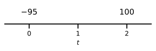
Therefore, every dollar paid in two years today costs $0.95. Thus, a bond that pays for certain $50,000 in two years today should cost 0.95 \times 50{,}000 = \$47{,}500.

Figure 2: Price and cash flows of a zero-coupon bond with face value $50,000 and expiring in 2 years.

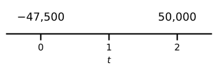
What if this new bond trades for a different price, say $47,000? Then, there would be an arbitrage opportunity. Note that 500 bonds paying $100 in two years are equivalent to a single bond paying $50,000 in two years. Therefore, buying the bond with a face value $50,000 expiring in two years and short-selling 500 bonds with a face value $100 expiring on the same date makes sense. This long-short strategy would provide today with a cash flow of $500 and, in two years, requires us to pay $50,000 for the bonds that we sold-short, which is precisely offset by the bond we bought.

Selling an asset short involves borrowing the asset first, which requires us to repay it later. Short-selling zero-coupon bonds may be more challenging for a small investor, but it will be easy for a prominent institutional investor such as a hedge fund.

Also, making $500 in one trade is not a large sum, but the idea here is to lever the transaction as much as possible. In principle the trade needs no money of your own, since the short sale pays for the purchase. In practice, brokers and repo lenders require collateral on both legs, so your capital limits how far you can scale the trade. If your arbitrage capital is $100 million, you can short-sell 1,000,000 bonds with face value $100 and purchase 2,000 bonds with face value $50,000 expiring in two years. The arbitrage profit gets amplified by 2,000, so you make $1,000,000 in the trade.

Arbitrage opportunities cannot last long as they generate free money for those exploiting them. The asset sold short should decrease in value, whereas the price of the asset bought should increase. Therefore, without arbitrage opportunities, the bond price with face value $50,000 must be $47,500.

We can also express the fact that $100 paid in two years costs today $95 as a percentage rate of return per year. Indeed, it must be the case that 95 (1 + r)^{2} = 100, if the annualized rate of return is r. Therefore, r = \left( \frac{100}{95} \right)^{1/2} - 1 = 2.60\%. In other words, the implicit interest rate paid by the 2-year zero coupon bond is 2.60% per year compounded annually.

As we can see, interest rates are usually derived from bond prices, although some interest rates are set directly in loans. The arbitrage opportunity we analyzed previously allowed us to borrow money at 2.60% and invest it at a higher rate.

In our example, the 2-year bond is free of the risk of default. We say that the 2-year risk-free rate is 2.60% per year. Risk-free rates for different maturities are fundamental to price derivatives. Therefore, it is essential to have a good proxy for them. In the next section, I review several types of interest rates found in financial markets and discuss which is the best proxy to use as a risk-free rate in pricing futures, forwards, and options.

Different Types of Interest Rates

Treasury Rates

The United States government issues Bills, Notes, and Bonds through the Department of the Treasury to finance government activities. The demand for Treasury securities is high since, for many investors, Treasury bonds represent an investment free of default risk.

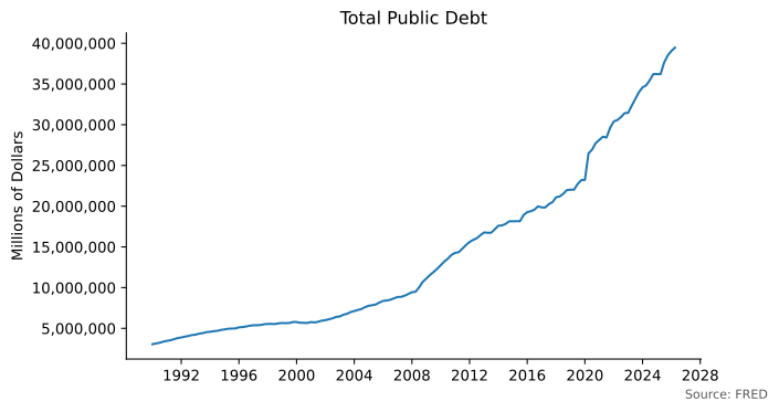
As of April 2026, the total public Treasury debt outstanding is $39.46 trillion. Let’s compare this figure with the market capitalization of the U.S. stock market, which is $69.0 trillion as of January 2026. It makes the U.S. Treasury debt market a big contender for worldwide investors.

Figure 3: The figure shows the evolution of the Treasury public debt from January 1990 until April 2026.

Notwithstanding the sheer size of the U.S. Treasury market, Treasury yields are not clean measures of the risk-free rate. They reflect the value investors place on the safety and liquidity of Treasuries, the demand from institutions that must hold them for regulatory reasons, and the supply of new debt. As a result, Treasury yields can differ from other benchmark rates in either direction: Treasury bills have historically yielded less than repo loans, while since 2015 the 10-year Treasury yield has been above the 10-year swap rate, even though those swaps referenced LIBOR, an unsecured bank rate. Therefore, Treasury rates are commonly not used as benchmark rates to price derivative securities.

LIBOR

LIBOR rates have been at the heart of the financial system for many decades. The acronym stands for London Interbank Offered Rate. For all this time, LIBOR has provided a reference for pricing derivatives, loans, and securities.

From the beginning, banks designed LIBOR to proxy for unsecured short-term borrowing between them, with tenors ranging from one day to one year. Also, LIBOR rates existed for different currencies.

Banks used to index large corporate loans to LIBOR. A company that would borrow money from a bank would then reimburse the loan by making quarterly payments indexed to the applicable three-month LIBOR. Many corporate borrowers, however, like to pay a fixed interest instead. Transforming a floating interest rate into a fixed one is possible by combining the loan with an interest rate swap. Thus, interest rate swaps were one of the most essential derivatives that used LIBOR as a reference rate.

In response to recommendations and objectives set forth by the Financial Stability Board and the Financial Stability Oversight Council to address risks related to USD LIBOR, the Federal Reserve Board and the New York Fed jointly convened in 2014 the Alternative Reference Rates Committee (ARRC), which is a group of private-market participants whose role is to ensure a successful transition from U.S. dollar (USD) LIBOR to a more robust reference rate. The recommended alternative was the Secured Overnight Financing Rate (SOFR). Duffie and Stein (2015) present a good summary and analysis of the reform.

Duffie, Darrell, and Jeremy C. Stein. 2015. “Reforming LIBOR and Other Financial Market Benchmarks.” Journal of Economic Perspectives 29 (2): 191–212.

There were two important reasons to abandon USD LIBOR in favor of SOFR. First, several cases of attempted market manipulation and false reporting of LIBOR came to light in 2012. Second, unsecured interbank borrowing became thin after the financial crisis of 2008, so LIBOR submissions rested largely on banks’ judgment rather than on actual transactions (Duffie and Stein 2015).

USD LIBOR has been discontinued and replaced by SOFR. The panel-based rates ended on June 30, 2023, and a synthetic version kept for legacy contracts ended in September 2024.

OIS and Overnight Rates

In the United States, banks hold reserve balances at the Federal Reserve and lend them to each other overnight in the federal funds market, where the Federal Home Loan Banks are also major lenders. Reserve requirements have been zero since March 2020, but institutions still trade reserves to manage their liquidity. The volume-weighted median rate of these overnight loans is termed the effective federal funds rate (EFFR).

Figure 4: The figure shows the evolution of the effective federal funds rate from January 1960 until September 2026.

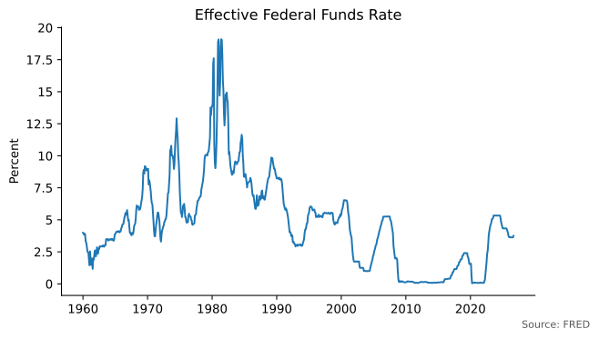
We can observe from the figure that there have been periods in which the federal funds rate has been very high, reaching almost 20% per year. From 2009 until late 2015, the federal funds rate was nearly zero.

When the Federal Reserve determines the target federal funds rate, it implements its policy by ensuring the EFFR is close to its target daily. Since December 2008, the Fed has maintained the EFFR between lower and upper limits, as the following figure shows.

Figure 5: The Federal Reserve makes sure that the EFFR stays within the target range. The figure shows the evolution of the EFFR starting in 2009.

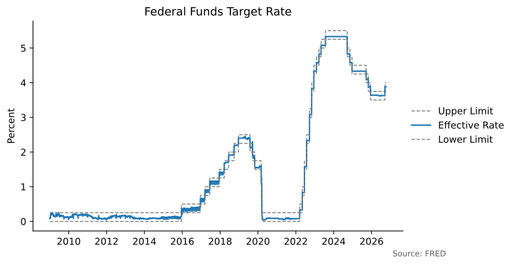
In March 2020, the COVID-19 pandemic pushed these limits back to zero, where they had been after the financial crisis of 2008. The inflation surge of 2021 and 2022 led the Federal Reserve to raise the target range to between 5.25% and 5.50% by July 2023, and it has been cutting rates since September 2024.

Traditionally, practitioners have used LIBOR and LIBOR-swap rates as proxies for risk-free rates when valuing derivatives. The financial crisis of 2007 put this practice into question. Banks became reluctant to lend to each other, and the TED spread, the difference between the 3-month LIBOR and the 3-month Treasury rate, surged significantly above its average level. It was clear that LIBOR was capturing the credit risk of the underlying banks and, therefore, could not be used to proxy for the risk-free rate.

The alternative chosen by practitioners was the overnight indexed swap rate. An overnight indexed swap (OIS) is an over-the-counter financial contract in which one party pays the compounded EFFR over a certain period, say three months, in exchange for a fixed payment. After the financial crisis of 2008, the OIS rate became the standard proxy for the risk-free rate (Hull and White 2015). The ARRC, however, preferred SOFR, because the repo market behind it is far larger than the federal funds market. In October 2020, the main clearinghouses switched the discounting of cleared U.S. dollar swaps from the EFFR to SOFR.

Hull, John C., and Alan White. 2015. “OIS Discounting, Interest Rate Derivatives, and the Modeling of Stochastic Interest Rate Spreads.” Journal of Investment Management 13 (1): 64–83.

SOFR and Repo Rates

In a repurchase agreement or repo, a financial institution or trader sells some securities to a counterparty with the agreement to repurchase them later for a slightly higher price. The implicit interest rate in this transaction is the repo rate. Unlike LIBOR and the EFFR, repo rates are secured borrowing rates.

The volume-weighted median rate of overnight repo transactions backed by Treasury securities is called the secured overnight financing rate (SOFR). U.S. regulators told banks to stop writing new LIBOR contracts after 2021, and SOFR has since replaced USD LIBOR.

Figure 6: The figure shows the evolution of the secured overnight financing rate (SOFR) from January 2019 until October 2026.

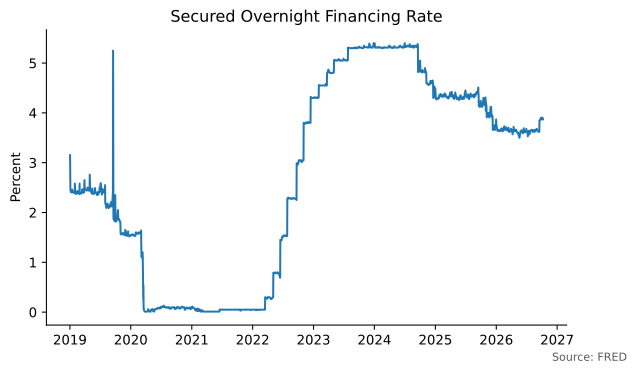
Given its close connection to secured overnight borrowing in a deep and liquid market, SOFR is the benchmark risk-free rate we will use throughout this course when pricing futures, forwards, and options.

Compounding Frequencies

The notion of future value (FV) is fundamental to finance. It allows us to compute how an investment grows over time when you apply a specific rate of interest to it. Unless otherwise stated, we will express all interest rates as a percentage per year. It makes a difference how often you compound the interest rate.

Example 1 (Annual compounding) If the interest rate is 10% per year compounded annually, after a year, $100 invested at this rate will grow to \text{FV} = 100 \times 1.10 = \$110.00.

In other words, the future value of $100 after a year is $110 when the interest rate is 10% per year with annual compounding. Consequently, a rate of 10% per year with yearly compounding corresponds to the investment’s effective annual rate (EAR).

A prevalent way to express the interest rate is with annual compounding. However, practitioners use other ways to express the interest rate in practice. For example, most bonds in the United States, including Treasury and corporate bonds, pay coupons every six months. Consequently, expressing the yield-to-maturity (YTM) of Treasury or corporate bonds with semi-annual compounding is very common. In this case, we divide the interest rate by two and compound it twice yearly.

Example 2 (Compounding different frequencies) If the interest rate is 10% per year compounded semi-annually, $100 will grow to \text{FV} = 100 \times 1.05^{2} = \$110.25. If that interest rate is 10% per year compounded monthly, $100 will grow to \text{FV} = 100 \left(1 + \frac{0.10}{12} \right)^{12} = \$110.47. If the same interest rate is compounded daily, $100 will grow to \text{FV} = 100 \left( 1 + \frac{0.10}{365} \right)^{365} = \$110.52. You could keep increasing the compounding frequency to see what happens with the future value.

Example 2 suggests the following rule for the EAR of an investment that uses a specific compounding rule.

WarningEffective Annual Rate

An interest rate r that is compounded n times per year will generate an effective annual rate equal to: \text{EAR} = \left(1 + \frac{r}{n}\right)^{n} - 1

The property implies that the EAR increases as we compound more often. It is also common to need to convert a rate from one compounding convention to another. To do so, equate the future values implied by each convention.

WarningConverting Between Compounding Conventions

To convert a rate r_m compounded m times per year to a rate r_n compounded n times per year, equate their future values: \left(1 + \frac{r_m}{m}\right)^{m} = \left(1 + \frac{r_n}{n}\right)^{n}. To convert to a continuously-compounded rate r_c, take the limit n \to \infty: \left(1 + \frac{r_m}{m}\right)^{m} = e^{r_c} \Rightarrow r_c = m \ln\!\left(1 + \frac{r_m}{m}\right).

Continuous Compounding

When pricing futures, forwards, options, and other derivatives, it is helpful to use continuous compounding to discount cash flows. In this section, we will learn how to use continuously compounded rates to compute present and future values.

Indeed, there is a limit to the compounding operation in Example 2: \lim_{n\rightarrow\infty} 100\left(1+\frac{0.10}{n}\right)^{n} = 100e^{0.10} = \$110.52. We call this operation continuous compounding, and compounding the interest rate daily is already a pretty good approximation of it. In a spreadsheet, to compute 100 e^{0.10} you need to type =100*exp(0.10).

More generally, an amount PV invested today in a risk-free deposit account earning an annual interest rate r compounded continuously will grow to FV = PV e^{r t} at time t.

Figure 7: Future value of PV invested at a continuously compounded rate r for time t.

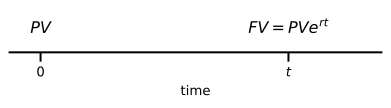
We say that FV is the future value of PV at time t. Equivalently, we say that PV = FV e^{-r t} is the present value of FV.

WarningContinuously-Compounded Interest Rate

If we denote by r the continuously-compounded interest rate, the relationship between present value (PV) and future value (FV) is given by: FV = PV e^{r T} \Longleftrightarrow PV = FV e^{-r T}.

Example 3 (Computing a future value) If you invest $500 at 6% per year with continuous compounding, in 16 months the balance of your account will be: FV = 500 e^{0.06 \times 16/12} = \$541.64. To perform the previous computation using a spreadsheet software you need to type =500*exp(0.06*16/12).

Example 4 (Computing a present value) You want to know how much you need to have in a bank account today so that in 18 months from now your balance is $2,000. The interest rate is 7% per year with continuous compounding.

The required amount is the present value of $2,000 for 18 months at 7%: PV = 2000 e^{-0.07 \times 18/12} = \$1{,}800.65. To perform the previous computation using a spreadsheet software you need to type =2000*exp(-0.07*18/12).

Example 5 (Computing a continuously compounded rate) Say that you invest $100 in a deposit account and after a year your balance is $110. What equivalent continuously compounded interest rate would give you the same amount?

If we denote by r the continuously compounded interest rate, it must be the case that: 110 = 100e^{r} \Rightarrow r = \ln\left(\frac{110}{100}\right) = 9.53\%. To perform the previous computation using a spreadsheet software you need to type =ln(110/100).

Therefore 10% per year compounded annually is the same as 9.53% per year compounded continuously.

Zero Rates

A zero-coupon bond pays its principal or face-value F at maturity but makes no intermediate payments.

Figure 8: The cashflows of a zero-coupon bond with face value F and expiring at time T.

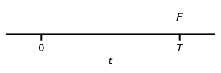
Apart from Treasury bills and Treasury STRIPS, zero-coupon bonds are not common in financial markets, but it is possible to synthesize a zero-coupon bond from a portfolio of two coupon bonds. For example, consider two coupon bonds with the same maturity T and coupon dates but different coupon rates. By taking a long position in one and a short position in the other in the right proportions, all intermediate coupon payments cancel, leaving only a single cash flow at maturity T. The resulting portfolio is equivalent to a zero-coupon bond maturing at T.

The price of a zero-coupon bond is determined by discounting its face-value at the relevant interest rate. For a given maturity T, the T-year zero rate, denoted by r(T), is the interest rate that gives the right T-year zero-coupon bond price Z(T). That is, if r(T) is a continuously-compounded rate we must have: Z(T) = F e^{-r(T) T}.

Example 6 (Computing the price of a zero coupon bond) You have the following information for zero rates expressed per year with continuous compounding:

Maturity (months)	1	3	6	9	12
Zero Rate (%)	6.0	6.4	6.6	6.8	7.0

Consider a zero-coupon risk-free bond with face value $1,000 and expiring in 9 months. To compute the price of the bond, we use the 9-month interest rate which is 6.8%: Z = 1000e^{-0.068 \times 9/12} = \$950.28.

Example 7 (Computing a zero rate) A 7-year zero-coupon risk-free bond with face value $1,000 trades for $650. The 7-year zero rate r expressed with continuous compounding satisfies: \begin{aligned} 1000 e^{-r \times 7} & = 650 \\ e^{-r \times 7} & = \frac{650}{1000} \\ -r \times 7 & = \ln\left(\frac{650}{1000}\right) \\ r & = -\frac{1}{7} \ln\left(\frac{650}{1000}\right) \end{aligned} The 7-year zero rate is then 6.15% per year with continuous compounding.

Practice Problems

Problem 1 You invest $5,000 at 15% per year with continuous compounding. How much will you have in the account after 14 years?

Solution

The balance in the account will be 5{,}000 e^{0.15 \times 14} = \$40{,}830.85 after 14 years.

Problem 2 Consider the following cash flows occurring at the times indicated below:

Time (years)	7	14	21
Cash flow	149	240	184

Compute the present value if the discount rate is 9% per year with continuous compounding.

Solution

The present value of these cash flows is: \textit{PV} = 149 e^{-0.09 \times 7} + 240 e^{-0.09 \times 14} + 184 e^{-0.09 \times 21} = 175.23.

Problem 3 The interest rate is 8% per year continuously-compounded and assumed to remain constant. Compute the present value of the following cash flows.

Time (years)	2	5	14	19
Cash Flow	100	200	300	150

Solution

\textit{PV} = 100 e^{-0.08 \times 2} + 200 e^{-0.08 \times 5} + 300 e^{-0.08 \times 14} + 150 e^{-0.08 \times 19} = \$349.97

Problem 4 An investor receives $1,100 in one year in return for an investment of $1,000 now. Calculate the percentage return per year with:

1. Annual compounding
2. Semiannual compounding
3. Monthly compounding
4. Continuous compounding

Solution

1. Annual compounding: 1,100 = 1,000 (1 + r) \Rightarrow r = \frac{1,100}{1,000} - 1 = 10\%
2. Semiannual compounding: 1,100 = 1,000 \left(1 + \frac{r}{2}\right)^{2} \Rightarrow r = 2 \left(\left(\frac{1,100}{1,000}\right)^{\frac{1}{2}} - 1\right) = 9.76\%
3. Monthly compounding: 1,100 = 1,000 \left(1 + \frac{r}{12}\right)^{12} \Rightarrow r = 12 \left(\left(\frac{1,100}{1,000}\right)^{\frac{1}{12}} - 1\right) = 9.57\%
4. Continuous compounding: 1,100 = 1,000 e^{r} \Rightarrow r = \ln\left(\frac{1,100}{1,000}\right) = 9.53\%

Problem 5 An effective annual rate (EAR) of 11% per year is equivalent to which rate expressed per year with continuous compounding?

Solution

1.11 = e^{r} \Rightarrow r = \ln(1.11) = 10.44\%.

Problem 6 You are considering an investment of $100 today that should grow to $167 in 8 years. What rate of return, expressed per year with continuous compounding, is consistent with this information?

Solution

100 e^{r \times 8} = 167 \Rightarrow r = \frac{1}{8} \ln\left(\frac{167}{100}\right) = 6.41\%

Problem 7 A bank quotes an interest rate of 14% per year with quarterly compounding. Compute an equivalent rate with:

1. Continuous compounding
2. Annual compounding

Solution

1. Continuous compounding: \left(1 + \frac{0.14}{4}\right)^{4} = e^{r} \Rightarrow r = 4 \ln\left(1 + \frac{0.14}{4}\right) = 13.76\%
2. Annual compounding: \left(1 + \frac{0.14}{4}\right)^{4} = 1 + r \Rightarrow r = \left(1 + \frac{0.14}{4}\right)^{4} - 1 = 14.75\%

Problem 8 A deposit account pays 12% per year with continuous compounding, but interest is actually paid quarterly. How much interest will be paid each quarter on a $10,000 deposit?

Solution

The interest paid quarterly should be 10,000 e^{0.12 \times 0.25} - 10,000 = \$304.55.

Problem 9 Suppose that 6-month, 12-month, 18-month, 24-month, and 30-month zero rates are, respectively, 4.0%, 4.2%, 4.4%, 4.6%, and 4.8% per year, with continuous compounding. Estimate the cash price of a bond with a face value of $100 that will mature in 30 months and pays a coupon of 4% per year semiannually.

Solution

B = 2 e^{-0.040 \times 0.5} + 2e^{-0.042 \times 1.0} + 2 e^{-0.044 \times 1.5} + 2 e^{-0.046 \times 2.0} + 102 e^{-0.048 \times 2.5} = \$98.04.

Problem 10 You have information of cash flows and zero-coupon rates (per year with continuous compounding) for different maturities as shown below:

Time (years)	4	10	17
Zero-coupon rate (%)	5.8	6.9	7.3
Cash flow	387	473	276

Compute the present value of those cash flows.

Solution

The present value of these cash flows is: \textit{PV} = 387 e^{-0.058 \times 4} + 473 e^{-0.069 \times 10} + 276 e^{-0.073 \times 17} = 623.91.