Forward and Futures Prices
No-Arbitrage
Forward and Futures Markets defined the forward price as the delivery price that makes a new forward contract worth zero. We now ask what determines it. We compute the forward price by assuming that it is hard to make easy money without taking any risk in financial markets. We call this notion the principle of no-arbitrage.
An arbitrage is a strategy that either generates money today and never requires a payment later, or costs nothing today, never loses money, and pays something in at least some states of the world. Such a deal would not last for long: traders would exploit it at a massive scale until prices moved to eliminate it. The principle does not depend on the details of agents’ preferences. It only requires that investors prefer more money to less and that they can trade, including selling short, without large frictions.
Throughout this chapter we treat futures and forward prices with the same maturity as equal, so every result applies to both. Section 4 explains when the two differ.
What the Arbitrage Requires
Every arbitrage argument in this chapter compares a forward contract with a position in the underlying asset held until delivery. For the comparison to pin down the forward price, we must be able to buy the asset today, or borrow it and sell it short, carry the position until the delivery date at a known cost and without risk, and deliver. Stocks, stock indices, and freely convertible currencies meet this requirement. Holding them costs nothing, since they do not deteriorate and need no storage, and their only carry is a known dividend or interest rate. For these assets, the cash price is the spot price, and the forward price follows from the spot price by arbitrage.
When the asset cannot be carried this way, the forward price is not tied to the cash price. In that case, the carry in the forward price is no longer a property of the asset, such as a dividend we can forecast, but an implied rate read from market prices: the forward price and the spot rate for a currency, or futures prices of different maturities for a commodity. Currencies subject to capital controls are one example, and physical commodities are another. We study them in Section 3.
Assets That Can Be Carried
Non-Dividend Paying Assets
The argument is short. Buy one unit of the asset for S and sell it forward for F. At time T we deliver the asset and receive F, whatever the asset price is then. The strategy costs S today and pays F for sure at T, so it is a risk-free investment, and its cost must equal the present value of F, that is, S = F e^{-r T}. If the forward price were different, one of the two strategies in the examples below would make money for nothing.
Example 1 Suppose that the current price of a non-dividend-paying stock is $40, and the 3-month US$ interest rate is 5% per year with continuous compounding. The no-arbitrage forward price is: F = 40 e^{0.05 \times 0.25} = 40.50.
The following example shows what would happen if the forward price of the contract described in Example 1 was higher than $40.50. When an asset is trading for more than its fair price, it makes sense to sell it.
Example 2 Suppose that the current price of a non-dividend-paying stock is $40, the 3-month forward price is $43, and the 3-month US$ interest rate is 5% per year with continuous compounding. Is there an arbitrage opportunity?
The table below shows the cash flows that an investor would get today and in three months if she sells one forward contract, borrows the present value of $43 to be paid in three months, and buys the stock. Borrowing means a positive cash flow today and a negative cash flow in the future, whereas buying a stock means a negative cash flow today and a positive cash flow in the future when we sell the stock.
| t = 0 | t = 3/12 | |
|---|---|---|
| Short forward | 0.00 | 43 - S_{T} |
| Borrow | 42.47 | -43 |
| Long stock | -40.00 | S_{T} |
| Total | 2.47 | 0 |
The table shows that the cost of this strategy is negative $2.47, i.e., you would make money today by engaging in these transactions. Furthermore, today’s positive cash flow has zero risk since we can see that the cash flow in three months is zero. Since by selling the forward for $43, we can make an arbitrage profit, we conclude that the forward price, in this case, is too high.
We now focus on the case when the observed forward price is less than its fair price. If this were the case, buying the forward and short-selling the stock would make sense. To sell a stock short, your broker borrows the shares from another client and sells them in the market. Later, you buy the shares back and return them to the lender, and in the meantime you pay the lender any dividends the shares pay.
Example 3 Suppose that the current price of a non-dividend-paying stock is $40, the 3-month forward price is $39, and the 3-month US$ interest rate is 5% per year with continuous compounding. Is there an arbitrage opportunity?
The table below shows an investor’s cash flows today and in three months if she buys one forward contract, invests the present value of $39 to get that amount in three months, and sells the stock short.
| t = 0 | t = 3/12 | |
|---|---|---|
| Long forward | 0.00 | S_{T} - 39 |
| Invest | -38.52 | 39 |
| Short stock | 40.00 | -S_{T} |
| Total | 1.48 | 0 |
Again, the cost of this strategy is negative as it generates money today. As before, the trader faces no risk in three months. There is an arbitrage opportunity because the forward price is too low.
Assets Paying Cash Dividends
Many assets pay dividends or other cash income during the life of a forward contract. For example, the owner of a stock receives its quarterly dividends, whereas the holder of a long forward on the stock does not. The forward price needs to be adjusted accordingly.
Example 4 Consider a stock that currently trades at $50. Analysts expect the stock to pay dividends of $1.15 and $1.20 in two and five months, respectively. If the risk-free rate is 5% per year with continuous compounding, let us compute the six-month forward price.
For this, we need to compute the present value of the dividends. Even though, in practice, dividend payments are uncertain, we could assume they are known for short-term maturities, and hence, we can discount them using the risk-free rate. We have that D = 1.15 e^{-0.05 \times 2/12} + 1.20 e^{-0.05 \times 5/12} = 2.32. Therefore, F = (50 - 2.32) e^{0.05 \times 6/12} = 48.89.
The forward price we computed in Example 4 is the price that prevents any arbitrage opportunities. If the forward price differed, an arbitrageur could engage in the following strategy and make arbitrarily large risk-free profits.
Example 5 Consider the same stock described in Example 4. What would an arbitrageur do if the six-month forward price was $50.20?
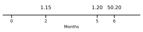
We know that the no-arbitrage forward price is $48.89. If the actual forward price is $50.20, it means that the six-month forward is too expensive, so we should sell it. We hedge the transaction by buying one share of the stock at $50. The timeline below shows what the arbitrageur receives: dividends in two and five months, and $50.20 in six months for delivering the share under the forward.
All this suggests that the arbitrageur could take the following loans to be repaid in full using the dividend payments and the sale of the stock in six months:
- Loan 1: Borrowing 1.15 e^{-0.05 \times 2/12} = \$1.14 today and repaying $1.15 in two months.
- Loan 2: Borrowing 1.20 e^{-0.05 \times 5/12} = \$1.18 today and repaying $1.20 in five months.
- Loan 3: Borrowing 50.20 e^{-0.05 \times 6/12} = \$48.96 today and repaying $50.20 in six months.
The table below describes the cash flows received by the arbitrageur when engaging in this transaction. A positive cash flow means the arbitrageur receives money, whereas a negative cash flow means the opposite.
| t = 0 | t = 2/12 | t = 5/12 | t = 6/12 | |
|---|---|---|---|---|
| Short forward | 0.00 | 50.20 - S_{T} | ||
| Loan 1 | 1.14 | -1.15 | ||
| Loan 2 | 1.18 | -1.20 | ||
| Loan 3 | 48.96 | -50.20 | ||
| Long stock | -50.00 | 1.15 | 1.20 | S_{T} |
| Total | 1.28 | 0 | 0 | 0 |
This strategy generates a sure profit of $1.28 per share of the stock and has no risk. An arbitrageur could sell 100 million forwards and hedge accordingly to generate an instantaneous risk-free profit of $128 million.
Assets Paying a Dividend Yield
Some assets behave as if they paid dividends continuously, like a stock index such as the S&P 500, whose many constituents pay dividends on different dates. In these cases, it is convenient to treat dividends as a percentage yield paid over time. We denote the continuously compounded dividend yield by \delta.
Over a short period \Delta t, each unit of the asset pays a dividend worth \delta \Delta t units of the asset. If we reinvest the dividends in the asset, our holding grows at the rate \delta, so one unit today becomes e^{\delta T} units at T.
The no-arbitrage argument follows the same logic as before. Buy e^{-\delta T} units of the asset for S e^{-\delta T} and reinvest the dividends in the asset, so that you hold exactly one unit at time T, and sell a forward. The strategy costs S e^{-\delta T} today and delivers F for sure at T, so its cost must equal F e^{-r T}, which gives F = S e^{(r - \delta) T}.
Index Futures
Futures contracts written on stock market indices are called index futures. There are index futures written on the S&P 500, Nasdaq-100, DAX, CAC 40, and Euro Stoxx 50, among many others. In general, index futures are very liquid and provide good trading opportunities for both speculators and hedgers.
Example 6 Consider an index tracking a portfolio of stocks that pays a dividend yield of 3% per year with continuous compounding. The index is currently at 4,300. The risk-free rate for all maturities is 1% per year continuously-compounded. The 6-month futures price can be computed as F = 4300 e^{(0.01-0.03) \times 6/12} = 4257.21. Note that because the dividend yield is higher than the risk-free rate, the futures price is less than the current spot price.
When the observed futures price deviates from this relationship, arbitrageurs trade the futures against the basket of stocks in the index, a strategy called index arbitrage. If F denotes the observed futures price:
- If F < S e^{(r - \delta) T} then you should buy the futures, sell e^{-\delta T} units of the index short and invest F e^{-r T} dollars in a risk-free money-market account.
- If F > S e^{(r - \delta) T} then you should sell the futures, buy e^{-\delta T} units of the index and borrow F e^{-r T} dollars.
In both cases the arbitrageur makes risk-free money today while being completely hedged when the futures reaches maturity. In the first case, the short seller owes the lender the dividends on the borrowed index. Paying them by borrowing and selling more of the index makes the short position grow from e^{-\delta T} units today to one unit at T, just as reinvested dividends make the long position in the second case grow to one unit.
If in Example 6 the 6-month futures is trading at 4,300, an arbitrageur could engage in the following transactions:
| t = 0 | t = 6/12 | |
|---|---|---|
| Short Futures | 0 | 4300 - S_{T} |
| Buy e^{-\delta T} units of the Index | -4235.98 | S_{T} |
| Borrow F e^{-r T} | 4278.55 | -4300 |
| Total | 42.57 | 0 |
The strategy generates a risk-free cash flow today of $42.57 per unit of the index sold forward, with no initial investment required. Actual index futures multiply the index by a contract size, $50 for the E-mini S&P 500, so the profit per contract would be 50 \times 42.57 = \$2{,}128.50, and an arbitrageur would trade many contracts. Index arbitrage keeps the futures price close to its no-arbitrage value.
Currency Forwards
An exchange rate is the price of one currency in units of another. The street convention for writing it can induce errors. The EUR/USD exchange rate, also written EUR-USD or EURUSD, is the number of US dollars (USD) per euro (EUR): a quote of 1.08 means \$1.08 \Leftrightarrow \text{€}1. The euro is the base currency, the asset being priced, and the dollar is the quote currency, the units of the price. Some textbooks write it the other way around.
Example 7 If the EUR/USD exchange rate is 1.08, for a US investor, 1 Euro is worth $1.08, but in Europe, how many euros is $1 worth? \frac{1}{1.08} = \text{€}0.93 \text{ per dollar}. Therefore, to buy $1, you must pay €0.93.
Some currency pairs, such as EUR/USD or GBP/USD, use the USD as the quote currency. However, most currency pairs use the dollar as the base currency, e.g., USD/JPY, USD/CNY, and USD/CLP.
Currency forwards trade over-the-counter, and the FX forward market is one of the largest in the world. The Triennial Survey of the Bank for International Settlements (BIS) reports a daily turnover in outright currency forwards of about $1.8 trillion in April 2025.
A unit of the base currency is an asset that pays a dividend yield: deposited in a bank, it earns the base currency’s interest rate. The forward price of a currency is therefore F = S e^{(r - r_{f}) T}, \tag{3} where S is the spot exchange rate, r is the interest rate of the quote currency, and r_{f} is the interest rate of the base currency, which plays the role of \delta. This relation is called covered interest parity. For USD/JPY, the dollar is the base currency, so r_{f} is the dollar rate and r is the yen rate.
Currency forward prices are usually quoted as forward points, which for most currency pairs are 10,000 times the difference between the forward and the spot price (100 times for pairs quoted in yen).
Example 8 The current GBP/USD exchange rate is 1.30. The interest rates in USD and GBP are 1% and 3% per year with continuous compounding, respectively. The 9-month GBP/USD forward price is then, F = 1.30 e^{(0.01 - 0.03) \times 9/12} = 1.28065, or 10{,}000 \times (1.28065 - 1.30000) = -193.5 forward points.
When the Underlying Cannot Be Carried
Non-Deliverable Forwards
The arbitrage behind covered interest parity requires an investor to convert dollars into the foreign currency today, hold a deposit in that currency until maturity, and convert back. Several countries restrict these transactions with capital controls, so that foreign investors cannot freely hold deposits in the local currency or move funds in and out. Examples include the Indian rupee, the Korean won, the Taiwan dollar, and the Brazilian real.
For these currencies, offshore investors trade non-deliverable forwards (NDFs). An NDF is a forward contract that is never delivered: at maturity, the parties exchange in dollars the difference between the contracted rate and an official fixing of the spot rate, multiplied by the notional amount. Since offshore investors cannot buy the currency, carry it, and deliver it, the NDF price is not tied to the onshore interest rate by arbitrage. It is set instead by the supply and demand of offshore hedgers and investors. The foreign interest rate implied by the NDF price, r_{f}^{*} = r - \frac{1}{T} \ln\left(\frac{F}{S}\right), can differ from the onshore interest rate for long periods. NDFs show in the cleanest form what happens when the underlying cannot be carried: the forward price becomes a market price in its own right, and the implied rate is an output of the market, not an input to a formula.
Example 9 The spot price of a currency subject to capital controls is $0.2000 per unit, the one-year NDF price is $0.1900, and the one-year dollar interest rate is 4% per year with continuous compounding. The foreign interest rate implied by the NDF price is r_{f}^{*} = 0.04 - \ln\left(\frac{0.1900}{0.2000}\right) = 9.13\%. Suppose the onshore deposit rate is 12%. Covered interest parity with the onshore rate would give a forward price of 0.2000 e^{(0.04 - 0.12)} = \$0.1846, below the NDF price. An investor who could buy the currency, deposit it onshore, and sell the NDF would make money, but capital controls prevent offshore investors from doing so, and the gap persists.
Commodity Futures
There are many futures written on commodities such as crude oil, copper, gold, and soybeans. As we saw in Forward and Futures Markets, the spot price of a commodity is the nearby futures price S_{t} = F(t, T_{1}). Deferred contracts are quoted against the nearby contract, and the futures curve itself is the primitive.
Buying the physical commodity, storing it, and delivering it against a futures contract is not risk free, because the basis moves, as Hedging the Basis shows. No arbitrage ties the futures curve to the cash price. Among futures contracts, though, no-arbitrage applies as for any traded asset: holding a futures position needs no storage, so the futures curve is the underlying against which spreads, options on futures, and other contracts are priced.
The spread between a deferred contract and the nearby contract is the price of storage between the two delivery dates. It equals the marginal cost of storing the commodity, including the interest on the money tied up in it, minus the marginal benefit of having stocks on hand, called the convenience yield. The spread is large when stocks are plentiful and can turn negative when they are scarce (Telser 1958). Gorton et al. (2013) find this pattern across 31 commodities from 1971 to 2010: the convenience yield falls as inventories rise, most sharply when inventories are low. It is convenient to summarize the spread with an implied yield \delta defined by F(t, T) = S_{t} e^{(r - \delta)(T - T_{1})}. Like the NDF rate, and unlike the dividend yield of a stock index, \delta is not a property of the commodity that we could measure and plug into a formula. It is read from futures prices, and it changes as the level of stocks changes. Gold is the case where storage is cheap and stocks are large, so its spreads are close to pure interest and its implied yield is close to zero.
Example 10 The nearby crude oil futures, expiring in one month, trades at $95 per barrel, and the contract expiring in one year trades at $93. The interest rate is 5% per year with continuous compounding. The implied yield between the two contracts is \delta = 0.05 - \frac{1}{11/12} \ln\left(\frac{93}{95}\right) = 7.32\%. The implied yield is higher than the interest rate, so the futures curve slopes down. The market is paying for oil now rather than later, a sign that stocks are scarce.
Negative Oil Prices
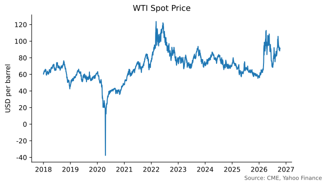
The COVID-19 pandemic hit countries hard in March 2020. As many economies came to a halt, crude inventories rose and storage at Cushing, Oklahoma, the delivery point of the NYMEX light sweet crude oil contract, was filling up. The buyer of a May 2020 contract is required, if the contract reaches maturity, to take delivery of 1,000 barrels of oil at Cushing. On April 20, 2020, the day before the contract expired, many traders still held long positions they did not want to take into delivery. To get out of a long futures position, you sell the same contract, but someone must be willing to buy it, and almost nobody wanted to, since buying meant taking oil with no place to store it.
The sellers ended up paying buyers to take the contracts, and the May contract, then the spot price, settled at about negative $38 a barrel. Figure 1 shows the spot price of oil since January 2018. The June contract settled that day at about $20, so the spread between the two contracts was about $58 a barrel: the price of storing oil at Cushing for one month, at a time when there was almost no storage left. The traders who paid to get out had done what almost nobody in futures markets does: they had carried a long position close to delivery without any place to store the oil.
A negative price is subtler than it looks. A claim that its owner can abandon at no cost never has a negative price, since nobody pays to give away what they could simply walk away from. Limited liability is this kind of free disposal for a stock, and it is why stock prices cannot fall below zero. The long futures had no such protection: it was an obligation to take delivery and pay, and the oil delivered at Cushing could not be thrown away either, since storage was full and dumping crude is illegal. Oil at Cushing on that date was a liability, and the expiring contract converged to its negative value. Electricity, which cannot be stored, reaches negative prices routinely for the same reason. Pricing models that assume prices stay positive, such as the lognormal model of later chapters, broke down, and CME switched its crude oil options to the Bachelier model, which allows negative prices.
Forwards vs. Futures
A forward contract is worth zero at inception. Later, it may have a positive or negative value since the underlying asset might increase or decrease in value, and the time-to-maturity of the contract decreases.
Suppose you entered a long forward some time ago with delivery price K, and you would like to know how much that contract is worth today. If the current forward price for the same maturity is F, you could enter a short forward today and completely hedge your future exposure. Indeed, in the past, you committed to purchasing the asset for K at maturity, but you just committed to selling it for F on the same date. You have just locked in a certain cash flow of F - K at time T, which in present value terms is worth today (F - K) e^{-r T}, where T is now the remaining time to maturity.
To value an existing short forward position entered some time ago at a forward price of K, you could buy a forward contract at F today, locking in a certain cash flow of K - F at maturity. The value of the short forward contract is then (K - F) e^{-r T}.
Example 11 You entered into a short forward contract some time ago at a forward price of $200. Today, the contract has six months until maturity, and the current forward price is $190. Also, the current risk-free rate is 5% per year with continuous compounding.
To compute the current value of the short forward position, we could imagine what would happen if we buy a forward today. That would lock in a sure cash flow in six months of 200 - 190 = \$10, whose present value today is 10 e^{-0.05 \times 6/12} = \$9.75, the value of the short forward contract.
These formulas apply to forwards. A futures position is marked to market every day, so after each settlement it is worth zero: the gains and losses that a forward accumulates in its value are paid out in cash through the margin account. When interest rates are deterministic, this difference in timing does not matter, and futures and forward prices with the same maturity are equal. This is the assumption we use in this chapter and in the option pricing chapters, so we refer to a futures or a forward contract interchangeably unless stated otherwise.
When interest rates are stochastic, the two prices differ by an amount that depends on how futures prices move with interest rates. If the futures price tends to rise when rates rise, the long futures receives its gains when rates are high and can reinvest them at those rates, and pays its losses when rates are low and can borrow cheaply. Daily settlement then favors the long, so the futures price is higher than the forward price. A negative correlation makes it lower, as is the case for SOFR futures, where the futures price (100 - rate) falls when rates rise.
For interest rate futures the difference is large enough to matter, and traders adjust the observed futures rate to obtain the forward rate. The correction is called a convexity adjustment.
Futures Prices vs. Expected Future Spot Prices
Many practitioners and academics have suggested that we could use futures or forward prices to forecast future spot prices. Since a futures price is the price at which buyers and sellers agree today to trade in the future, it seems natural that their forecasts would show up in it.
Whether futures prices are unbiased predictors of future spot prices depends on whether investors require a risk premium to hold the asset. A clean way to think about the question is to ask what discount rate investors apply to the asset.
Suppose that \mu is the rate at which investors discount a claim to one unit of the asset at time T. The excess \mu - r is the risk premium, whatever its source: how much the price moves with the market as a whole, or a premium hedgers pay speculators to bear their risk. Denote by F the futures price for delivery at time T. Imagine that you want to compute the value of 1 unit of the asset paid at time T. You could do this in two different ways. Either you discount the expected value of the asset at \mu, or you hedge your exposure by selling a futures, which provides a certain cash flow F that can then be discounted at the risk-free rate. Therefore, F e^{-r T} = \operatorname{E}(S_{T}) e^{-\mu T}, or F = \operatorname{E}(S_{T}) e^{(r - \mu) T}.
The previous expression shows that futures prices are unbiased predictors of expected future spot prices only when the asset carries no risk premium. More generally, futures prices will under- or over-estimate expected future spot prices depending on the sign of the risk premium \mu - r, as shown in the table below.
| Risk Premium | Expected Return | Futures vs. Expected Price |
|---|---|---|
| Zero | \mu = r | F = \operatorname{E}(S_{T}) |
| Positive | \mu > r | F < \operatorname{E}(S_{T}) |
| Negative | \mu < r | F > \operatorname{E}(S_{T}) |
Determining the risk premium of a commodity is not an easy task in practice, and the evidence has been debated for almost a century. Keynes (1930) and Hicks (1939) argued that hedgers are net short and pay speculators to bear their risk, so that \mu > r and the futures price sits below the expected spot price. Working (1953) argued instead that most hedgers are merchants trading the basis rather than buyers of insurance, the view developed in Hedging the Basis. Telser (1958) tested the Keynes-Hicks view directly. If hedgers paid a premium, futures prices would drift upward as contracts approach maturity, and cotton and wheat futures from 1926 to 1954 show no such trend once changes in the general price level are accounted for. Cootner (1960) replied that hedging is net short only after the harvest, when merchants hold large inventories, and can be net long before it, so the sign of \mu - r changes over the season. Futures prices should then fall while hedges build up and rise once they are lifted, and he finds this pattern in wheat futures in Telser’s own sample years.
Keynes, John Maynard. 1930. A Treatise on Money. Macmillan.
Hicks, John R. 1939. Value and Capital. Clarendon Press.
Working, Holbrook. 1953. “Futures Trading and Hedging.” American Economic Review 43 (3): 314–43.
Telser, Lester G. 1958. “Futures Trading and the Storage of Cotton and Wheat.” Journal of Political Economy 66 (3): 233–55.
Cootner, Paul H. 1960. “Returns to Speculators: Telser Versus Keynes.” Journal of Political Economy 68 (4): 396–404.
Dusak, Katherine. 1973. “Futures Trading and Investor Returns: An Investigation of Commodity Market Risk Premiums.” Journal of Political Economy 81 (6): 1387–406.
Bessembinder, Hendrik. 1992. “Systematic Risk, Hedging Pressure, and Risk Premiums in Futures Markets.” Review of Financial Studies 5 (4): 637–67.
Gorton, Gary B., Fumio Hayashi, and K. Geert Rouwenhorst. 2013. “The Fundamentals of Commodity Futures Returns.” Review of Finance 17 (1): 35–105.
Dusak (1973) reads the formula above through the CAPM: \mu - r depends on how the price moves with total wealth, not on its variability. For wheat, corn, and soybean futures from 1952 to 1967 she finds systematic risk and average returns both close to zero, the first row of the table. Bessembinder (1992) finds that returns on agricultural and currency futures still vary with hedgers’ net positions after controlling for systematic risk, which supports hedging pressure as a source of the premium. Gorton et al. (2013) find instead that the premium varies with inventories, with low-inventory commodities earning higher returns, while traders’ positions, the usual measure of hedging pressure, do not predict returns.
Practice Problems
Problem 1 Suppose you enter into a 6-month forward contract on a non-dividend-paying stock when the stock price is $30, and the risk-free interest rate is 12% per year with continuous compounding. What is the forward price?
Solution
F = 30 e^{0.12 \times 6/12} = 31.86.Problem 2 A non-dividend-paying stock trades at $25, the 6-month forward price is $26, and the 6-month interest rate is 4% per year with continuous compounding. Is there an arbitrage opportunity? If so, describe the strategy and the profit per share.
Solution
The no-arbitrage forward price is 25 e^{0.04 \times 6/12} = 25.51, so the forward at $26 is too expensive. Sell the forward, buy the stock for $25, and borrow 26 e^{-0.04 \times 6/12} = 25.49. In six months, deliver the stock for $26 and repay the loan. The strategy earns 25.49 - 25 = \$0.49 per share today with no cash flow later.Problem 3 A stock trades at $60 and will pay a dividend of $0.80 in three months. The risk-free rate is 4% per year with continuous compounding. What is the six-month forward price?
Solution
D = 0.80 e^{-0.04 \times 3/12} = 0.79, \qquad F = (60 - 0.79) e^{0.04 \times 6/12} = 60.40.Problem 4 A 1-year long forward contract on a non-dividend-paying stock is entered into when the stock price is $40, and the risk-free rate of interest is 10% per annum with continuous compounding.
- What are the forward price and the initial value of the forward contract?
- Six months later, the price of the stock is $45, and the risk-free interest rate is still 10%. What are the forward price and the value of the forward contract?
Solution
- F = 40 e^{0.10 \times 1} = 44.21 and V = 0.
- F = 45 e^{0.10 \times 0.5} = 47.31 and V = (47.31 - 44.21) e^{-0.10 \times 0.5} = 2.95.
Problem 5 A stock index currently stands at 350. The risk-free interest rate is 8% per year with continuous compounding and the dividend yield on the index is 4% per year. What should be the futures price for a 4-month contract?
Solution
F = 350 e^{(0.08 - 0.04) \times 4/12} = 354.70.Problem 6 Assume that the risk-free interest rate is 9% per annum with continuous compounding and that the dividend yield on a stock index varies throughout the year. In February, May, August, and November, dividends are paid at a rate of 5% per annum. In other months, dividends are paid at a rate of 2% per annum. Suppose that the value of the index on July 31 is 1,300. What is the futures price for a contract deliverable on December 31 of the same year?
Solution
During the life of the contract, the index will pay dividends in August and November when the dividend yield is 5%, and in September, October and December when the dividend yield is 2%. Therefore, F = 1300 e^{0.09 \times 5/12 - (0.05 \times 2/12 + 0.02 \times 3/12)} = 1331.80.Problem 7 The EUR/USD exchange rate is 1.10. The one-year interest rates are 4% in dollars and 2% in euros, both with continuous compounding. What is the one-year EUR/USD forward price, and how many forward points is it?
Solution
The euro is the base currency, so r_{f} is the euro rate: F = 1.10 e^{(0.04 - 0.02) \times 1} = 1.12222, or 10{,}000 \times (1.12222 - 1.10000) = 222.2 forward points.Problem 8 A currency subject to capital controls trades at $0.0500 per unit. The 6-month non-deliverable forward price is $0.0495, and the 6-month dollar interest rate is 5% per year with continuous compounding. What foreign interest rate is implied by the NDF price?
Solution
r_{f}^{*} = 0.05 - \frac{1}{0.5} \ln\left(\frac{0.0495}{0.0500}\right) = 7.01\%.Problem 9 The nearby copper futures, expiring in one month, trades at $4.50 per pound, and the contract expiring in ten months trades at $4.60. The interest rate is 6% per year with continuous compounding. What implied yield does the spread between the two contracts imply? What does it suggest about copper stocks?