Financial Derivatives
Introduction
In this class we study the pricing, hedging, and uses of financial derivatives or derivatives for short. A derivative is a financial instrument whose value depends on the value of another asset, such as a stock, a foreign currency, a futures contract, or another quantity, such as volatility.
Futures and forward contracts are derivatives that allow traders to fix the price at which an asset will trade at a given date. In this sense, futures or forward contracts give the holder the obligation to buy or sell at a specific price, unlike options, which provide the holder with the right but not the obligation to buy or sell at a particular price.
Derivatives Contracts
As for any other financial instrument, the value of a derivative is the present value of its expected payoff. A positive payoff means receiving money, whereas a negative payoff represents an outflow of cash.
The payoff represents how much money you get if you buy the instrument. The profit, on the other hand, depends on how much you pay for the derivative. For many derivatives the payoff is realized at maturity, but not for all.1
1 American-type options can realize the payoff anytime before or at maturity.
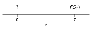
If S_{T} denotes the value of a stock at maturity, the payoff of a derivative written on the stock will be a function of S_{T} that we denote by f(S_{T}). An important question that we answer in this class is how to price this type of derivative.
If we denote by \xi the relevant continuously compounded discount rate for the derivative, the value of the derivative is V = e^{-\xi T} \operatorname{E}\left[f(S_{T})\right]. \tag{1} Even though this expression is correct, we do not generally know the right value for the discount rate \xi. For many derivatives, the only way to know \xi would be to know the value of the derivative first.2
2 For options, for example, the relevant discount rate under the historical or physical measure depends on the moneyness and the option’s maturity.
To circumvent this problem, the seminal work of Black and Scholes (1973) and Merton (1973) showed that it is possible to price derivatives by replication. Continuously trading in the underlying asset and a risk-free bond can generate the same payoffs as a derivative written on the asset. If that is the case, the value of the replicating portfolio today must be the value of the derivative asset to prevent arbitrage opportunities.
Their analysis also showed that the replicating strategy does not depend on the expected return of the underlying asset. Given the current price of the underlying asset, derivative prices therefore do not depend on that expected return or on the risk preferences that determine it. Since the expected return plays no role, we can price the derivative as if all assets were expected to earn the risk-free rate. This is what working under the risk-neutral probability measure means.
Under the risk-neutral probability measure, the value of the derivative is V = e^{-r T} \operatorname{E}^{*}\left[f(S_{T})\right] \tag{2} where r denotes the risk-free rate, and the expectation is taken under the risk-neutral probability measure.
A crucial difference between (1) and (2) is the discount rate used to price the derivative. In (1), we need to know both the expected return of the underlying asset, to compute the expectation, and the discount rate of the derivative, to compute its price. In (2), on the other hand, we can discount the expected payoffs of any asset at the risk-free rate.
The payoff function is linear for some derivatives, such as forward contracts, simplifying the expected payoff computation. For other derivatives, such as options, the payoff function is nonlinear and generally more complex to price than linear payoffs.
Example 1 (A derivative with a linear payoff) A forward contract is a commitment to purchase or sell an asset at maturity for K. The payoff of a long forward is the difference between the price of the asset at maturity and the price agreed in the contract; that is, the payoff is a linear function of the asset price at maturity: f(S_{T}) = S_{T} - K
Because the payoff can be positive or negative depending on the sign of S_{T} - K, the value of the contract can be positive or negative. Usually, the contract has zero value at inception. Later on, the value of the contract will change and might become positive or negative.
Example 2 (A derivative with a nonlinear payoff) A European option gives the holder the right but not the obligation to purchase or sell an asset at maturity for a given price of K. The payoff of an option is a nonlinear function of the asset price at maturity.
For example, the buyer of a call option receives: f(S_{T}) = \begin{cases} 0 & \text{if } S_{T} < K \\ S_{T} - K & \text{if } S_{T} \geq K \\ \end{cases}
Since the payoff is never negative and is positive in some states, the holder of an option must pay a premium to the seller.
More Complex Derivatives
The linear and nonlinear payoff structures illustrated above serve as the fundamental building blocks from which more complex instruments are constructed. The financial engineering revolution of the 1980s revolved around the idea that we could package these simpler derivatives to build new products. Pricing many more complex derivatives involves knowing how to price the basic building blocks used to make the financial product.
Derivatives with Periodic Payments
A classical way to create a more complex and helpful derivative is to put derivatives with different expirations together, creating a product that involves the payment of cash flows periodically over time.
For example, interest rate swaps involve the exchange of a fixed interest rate for a floating interest rate or vice-versa. They allow corporations to convert a floating-rate loan into a fixed-rate one. Another example is a credit default swap (CDS), in which one party makes periodic payments in exchange for protection in case a reference issuer defaults.
Pricing derivatives with periodic payments is similar to pricing a derivative with a single payment. If we denote by p(\cdot) the pricing functional, we have that p(f_{1}(S_{t_{1}}) + f_{2}(S_{t_{2}}) + \ldots + f_{n}(S_{t_{n}})) = p(f_{1}(S_{t_{1}})) + p(f_{2}(S_{t_{2}})) + \ldots + p(f_{n}(S_{t_{n}})), where f_{i}(S_{t_{i}}) is the payment at date t_{i}.
The same logic applies to the pricing of bonds. The price of a bond must be the sum of the present values of its coupons and its face value; otherwise, there would be a straightforward arbitrage opportunity. This follows from the law of one price, which says that two portfolios with the same payoffs must have the same price. In frictionless markets, the law of one price implies that pricing is linear.
Assets with Embedded Derivatives
Many assets, such as corporate bonds, have embedded options. For example, many bonds in financial markets are callable; the issuer has the right to repurchase the bond at a predetermined call price before maturity. Valuing a callable bond involves modeling the evolution of the term structure of interest rates and analyzing in which states it is profitable to call the bond.
For many callable bonds, the issuer has the right to call a bond at any time, starting on the first date the bond is callable until its maturity. Therefore, the call option embedded in these bonds is an American-type option. The pricing of these bonds requires using numerical techniques such as binomial trees since American-type options generally have no closed-form price. Because the issuer holds this valuable option, a callable bond trades at a lower price than an otherwise identical plain-vanilla bond.
Other bonds are convertible into shares of the issuing company at a fixed price. Thus, convertible bonds contain a call option on the company stock held by the bondholder. Because the bondholder holds this valuable option, a convertible bond trades at a higher price than an otherwise identical plain-vanilla bond.
Completing the Market
Theoretically, we could design a derivative with any payoff function f(S) that one might think of. For example, we could choose f(S) = S^{2} or f(S) = \ln(S).
With bonds, forwards, and options at every strike, it is possible to build any payoff that depends on the price of the underlying asset at a given maturity, including the two examples above. In this sense, options with different strikes complete the market. In practice only finitely many strikes trade, and combinations of options with different strikes and maturities, called options strategies, approximate the payoffs traders want.
Derivatives Markets
Uses of Derivatives
Derivatives allow investors to obtain payoffs that are useful to achieve specific objectives. For example, some commodity producers use derivatives to hedge their future production by fixing today the price at which they will sell. Other traders like derivatives because they can obtain custom-designed payoffs, allowing them to speculate in specific ways.
At given prices, derivatives make both types of traders, hedgers and speculators, better off by expanding their trading opportunity set.
Why a firm would hedge at all is less obvious than it seems. Shareholders can adjust their own exposure to commodity prices, so hedging inside the firm should add no value. Froot et al. (1993) argue that it does when outside financing costs more than internal funds: hedging keeps a drop in cash flow from forcing the firm to cut good investments.
The interaction between hedgers and speculators has been widely studied in commodity markets. Keynes (1930) and Hicks (1939) see speculators primarily as risk-takers who provide insurance to risk-averse hedgers, who pay premiums to speculators. Working (1953), in contrast, sees hedgers, mainly merchants and processors who hold inventories, as profit-seeking traders, for whom hedging is a form of arbitrage undertaken mostly in the expectation of a favorable change in the relation between cash and futures prices. Whether hedgers in fact pay speculators a premium is an empirical question we return to in Forward and Futures Prices.
The Market for Derivatives
Exchange-traded and over-the-counter derivatives are in zero-net supply: every long position has a corresponding short position. Some end users want long positions and others short ones, so their combined net demand can be positive or negative.
The demand for derivatives comes from buy-side traders who want to use derivatives for hedging or speculative purposes. For example, many hedgers in commodity markets are producers, merchants, and processors who want to fix the price at which they can sell their output or inventories. Hedging their exposure using futures involves selling these contracts to whoever is willing to take the opposite side of the trade.
The net demand, positive or negative, is balanced by sell-side investors or market makers that provide liquidity to the rest of the market.
Pricing and Hedging of Derivatives
Market makers hedge their exposure by dynamically trading the underlying asset and risk-free bonds. Since a perfectly hedged portfolio must earn the risk-free rate, this replication perspective is the main intuition behind the Black-Scholes model. The specific hedging strategy depends on how the underlying asset is modeled: whether time is discrete or continuous, and whether log returns are normally distributed or follow a richer process with stochastic volatility or jumps.
When perfect replication is not feasible, the pricing of derivatives might depend on supply and demand forces. For example, Garleanu et al. (2009) show how in an incomplete market the net demand for options can influence their price. The intuition for this result is simple. If risk-averse market makers cannot hedge all the risk of the trades they take on with customers, they ask for a risk compensation that grows with the net demand for the derivative and with the part of its risk that they cannot hedge.
Practice Problems
Problem 1 A trader enters a long forward contract on a stock. At maturity, the stock price is below the delivery price. What is the sign of the payoff? What is the sign of the profit if the contract had positive value at inception? Can the value of a forward contract be negative?
Solution
The payoff S_T - K < 0 is negative since S_T < K. If the contract had positive value at inception, the trader paid a premium, so the profit is even more negative than the payoff. Yes, the value of a forward contract can be negative: if the delivery price K is set above the fair forward price, the long position has negative value and the holder would need to be compensated to enter the contract.Problem 2 A company issues a callable bond and a convertible bond. For each, identify the embedded option, state who holds it, and explain why the embedded option affects the bond’s price relative to a plain-vanilla bond.
Solution
A callable bond embeds a call option held by the issuer and written by the bondholder: the issuer can repurchase the bond at a predetermined price before maturity. Because the issuer holds a valuable option, the callable bond trades at a lower price than an otherwise identical plain-vanilla bond. A convertible bond embeds a call option on the issuer’s stock held by the bondholder: the holder can convert the bond into shares at a fixed price. Because the bondholder holds a valuable option, the convertible bond trades at a higher price than an otherwise identical plain-vanilla bond.Problem 3 A derivative pays f(S_T) at maturity T. Write down the risk-neutral pricing formula and explain each component. Why can we discount expected payoffs at the risk-free rate r rather than at a higher rate that reflects the derivative’s risk?
Solution
The risk-neutral pricing formula is V = e^{-rT} \operatorname{E}^{*}[f(S_T)], where r is the risk-free rate, T is the time to maturity, and \operatorname{E}^{*} denotes the expectation under the risk-neutral probability measure. We can discount at r because, under the risk-neutral measure, all assets are expected to earn the risk-free rate by construction. This is not an assumption about investor preferences but a consequence of replication: since the derivative can be replicated by trading the underlying asset and a risk-free bond, its value must equal the cost of the replicating portfolio, which is given by today’s prices of the underlying asset and the bond.Problem 4 Explain the replication argument for pricing derivatives. Why does replication allow us to price a derivative without knowing investor risk preferences or the expected return on the underlying asset?