The Impact of Dividends

Published

October 14, 2026

Assets Paying Cash Dividends

Put-Call Parity with Dividends

For European options written on stocks paying cash dividends, the put-call parity is modified as follows: C - P = S - D - K e^{-r T} where D is the present value of dividends paid during the life of the option.

In order to derive this expression we will proceed as before by trying to build a covered call in two different ways. Suppose that we use the same two strategies as in Properties of European Options.

Strategy A: Long stock and short call \begin{aligned} \text{Cost} & = S - C \\ \text{Payoff} & = \begin{cases} S_{T} + \textit{FV}(D) & \text{if $S_{T} \leq K$} \\ K + \textit{FV}(D) & \text{if $S_{T} > K$} \end{cases} \end{aligned} Strategy B: Long bond and short put \begin{aligned} \text{Cost} & = K e^{-r T} - P \\ \text{Payoff} & = \begin{cases} S_{T} & \text{if $S_{T} \leq K$} \\ K & \text{if $S_{T} > K$} \end{cases} \end{aligned} We can see that both strategies no longer have the same payoff at maturity because the stock pays dividends. Let us then adjust the first strategy to account for the fact that the stock pays dividends.

Strategy A: Long stock, borrow D and short call \begin{aligned} \text{Cost} & = S - D - C \\ \text{Payoff} & = \begin{cases} S_{T} & \text{if $S_{T} \leq K$} \\ K & \text{if $S_{T} > K$} \end{cases} \end{aligned} Strategy B: Long bond and short put \begin{aligned} \text{Cost} & = K e^{-r T} - P \\ \text{Payoff} & = \begin{cases} S_{T} & \text{if $S_{T} \leq K$} \\ K & \text{if $S_{T} > K$} \end{cases} \end{aligned} Note that in A we use the dividends, reinvested at r, to repay the loan and generate the same payoff as in B.

Example 1 Suppose that S = 110, r = 5\%, K = 110, T = 9 months, and C = 13.30. The stock is expected to pay dividends of $2 in six months, and $2.5 in one year. What should be the no-arbitrage price of a European put with the same strike and maturity as the European call?

In order to use put-call parity to find the price of the European put, we need to compute the present value of the dividends that will be paid during the life of the option. Hence, we only consider the dividend that will be paid at t = 6/12 but not the dividend that will be paid at t = 1: D = 2 e^{-0.05 \times 6/12} = 1.95. Then, according to put-call parity we should have that a European put with the same strike and maturity as the call should cost: P = 13.30 - 110 + 1.95 + 110 e^{-0.05 \times 9/12} = 11.20. The put should then trade for $11.20.

Example 2 What if in the previous example everything stays the same, but you find that the put trades for $11?

Transactions	T = 0	T = 6/12	T = 9/12, S_{T} \leq 110	T = 9/12, S_{T} > 110
Long put	-11.00	0	110 - S_{T}	0
Short call	13.30	0	0	-(S_{T} - 110)
Long stock	-110.00	2	S_{T}	S_{T}
Borrow D	1.95	-2	0	0
Short bond	105.95	0	-110	-110
Total	0.20	0	0	0

Then we have an arbitrage opportunity since the put is relatively cheap compared to what it should trade. Hence, we should buy the put and sell the synthetic put. Note that the stock will pay a dividend of $2 in six months that can be used to pay the loan at that time.

Lower Bound on European Options with Dividends

With dividends, we modify the lower bounds on European call and put options as follows: \begin{aligned} C & \geq \max(S - D - K e^{-r T}, 0) \\ P & \geq \max(K e^{-r T} - S + D, 0) \end{aligned}

Example 3 Suppose that you have S = 110, r = 5\%, K = 110, and T = 9 months. The stock is expected to pay a dividend of $2 in six months, and of $2.5 in 1 year. The previous result implies that: C \geq \max(110 - 2e^{-0.05 \times 6/12} - 110 e^{-0.05 \times 0.75}, 0) = \max(2.10, 0) = 2.10 Hence, no matter how low the volatility is on this European call option with strike $110 and maturity 9 months, its premium must be higher than $2.10.

Assets Paying a Dividend Yield

The Dividend Yield

There are many assets that pay dividends continuously, like a currency, or that can be modeled as such, like a stock index. In these cases it is convenient to model dividends as a percentage yield paid over time. We will denote the continuously-compounded dividend yield by \delta.

Over each short interval \Delta t, the asset then pays a dividend of \delta S_{t} \Delta t. Therefore, the dividend yield can be seen as the units of the asset growing over time at the rate \delta. In practice, this is the approach used to model options on stock indices and currencies, although some practitioners also use it to model individual stocks as well.

Put-Call Parity and European Options Bounds

Put-Call Parity with a Dividend Yield

For European options written on assets paying a dividend yield, the put-call parity is modified as follows: C - P = S e^{-\delta T} - K e^{-r T} where \delta is the dividend yield paid continuously by the asset during the life of the option.

In order to derive this expression we will proceed as before by trying to build a covered call in two different ways.

Strategy A: Long e^{-\delta T} units of the asset and short call \begin{aligned} \text{Cost} & = S e^{-\delta T} - C \\ \text{Payoff} & = \begin{cases} S_{T} & \text{if $S_{T} \leq K$} \\ K & \text{if $S_{T} > K$} \end{cases} \end{aligned} Strategy B: Long bond and short put \begin{aligned} \text{Cost} & = K e^{-r T} - P \\ \text{Payoff} & = \begin{cases} S_{T} & \text{if $S_{T} \leq K$} \\ K & \text{if $S_{T} > K$} \end{cases} \end{aligned} Note that in A the asset grows at the rate \delta, so the total number of units of the asset at maturity is e^{-\delta T} e^{\delta T} = 1.

Example 4 Suppose that S = 110, r = 5\%, \delta = 3\%, K = 110, T = 9 months, and C = 13.30. What should be the no-arbitrage price of a European put with the same strike and maturity as the European call?

According to put-call parity we should have that a European put with the same strike and maturity as the call should cost: P = 13.30 - 110 e^{-0.03 \times 9/12} + 110 e^{-0.05 \times 9/12} = 11.70.

Example 5 What if in the previous example everything stays the same, but you find that the put trades for $11?

Transactions	T = 0	T = 9/12, S_{T} \leq 110	T = 9/12, S_{T} > 110
Long put	-11.00	110 - S_{T}	0
Short call	13.30	0	-(S_{T} - 110)
Long e^{-\delta T} units of asset	-107.55	S_{T}	S_{T}
Short bond	105.95	-110	-110
Total	0.70	0	0

Then we have an arbitrage opportunity since the put is relatively cheap compared to what it should trade. Hence, we should buy the put and sell the synthetic put. Note that because the asset pays a dividend yield we need to purchase slightly less of it today in order to get one unit if the asset in nine months.

Lower Bounds of European Options with Dividend Yields

If the asset pays a dividend yield, we modify the lower bounds on European call and put options as follows: \begin{aligned} C & \geq \max(S e^{-\delta T} - K e^{-r T}, 0) \\ P & \geq \max(K e^{-r T} - S e^{-\delta T}, 0) \end{aligned}

Example 6 Suppose that you have S = 110, r = 5\%, \delta = 3\%, K = 110, and T = 9 months. The previous result implies that: C \geq \max(110 e^{-0.03 \times 9/12} - 110 e^{-0.05 \times 9/12}, 0) = \max(1.60, 0) = 1.60 Hence, no matter how low the volatility is on this European call option with strike $110 and maturity 9 months, its premium must be higher than $1.60.

Since the payoffs of strategies A and B described above are positive, the cost of both strategies must be positive.

Upper Bounds of European Options with Dividend Yields

If the asset pays a dividend yield, the upper bounds on European call and put options are as follows: \begin{aligned} C & \leq S e^{-\delta T} \\ P & \leq K e^{-r T} \end{aligned}

Example 7 Suppose that you have S = 110, r = 5\%, \delta = 3\%, K = 110, and T = 9 months. The previous result implies that: C \leq 110 e^{-0.03 \times 9/12} = 107.55 Hence, no matter how high the volatility is on this European call option with strike $110 and maturity 9 months, its premium must be less than $107.55.

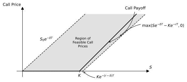
Feasible Prices for European Call Options

The graph describes the region of feasible prices for European call options written on an asset that pays a positive dividend yield such that \delta > r.

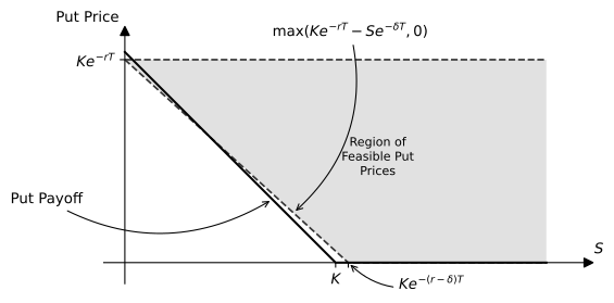
Call price against the stock price S for an asset paying a dividend yield. The shaded region of feasible prices lies between the upper bound, the dashed line S0 times e to the minus delta T, and the lower bound, the dashed line max of S times e to the minus delta T minus K times e to the minus rT, zero, which leaves zero at K times e to the minus r minus delta times T, to the right of K. The solid call payoff starts at K.

Feasible Prices for European Put Options

The graph describes the region of feasible prices for European put options written on an asset that pays a positive dividend yield such that \delta > r.

Put price against the stock price S for an asset paying a dividend yield. The shaded region of feasible prices lies between the upper bound, a dashed horizontal line at K times e to the minus rT, and the lower bound, the dashed line max of K times e to the minus rT minus S times e to the minus delta T, zero, which reaches zero at K times e to the minus r minus delta times T, to the right of K. The solid put payoff reaches zero at K.

Practice Problems

Problem 1 A four-month European call option on a dividend-paying stock is currently selling for $5. The stock price is $64, the strike price is $60, and a dividend of $0.80 is expected in one month. The risk-free interest rate is 12% per annum for all maturities. What opportunities are there for an arbitrageur?

Solution

We must have that: C \geq \max(64 - 0.80 e^{-0.12 \times 1/12} - 60 e^{-0.12 \times 4/12}, 0) = \$5.56. This means that the call is below the minimum price that forbids arbitrage, i.e. we can synthesize using put-call parity a European put option with the same strike and maturity but with a negative price. Remember that put-call parity says that: P = C - S + D + K e^{-r T} where D = 0.80 e^{-0.12 \times 1/12} = \$0.79 and K e^{-r T} = 60 e^{-0.12 \times 4/12} = \$57.65. We can then proceed as follows:

Transactions	T = 0	T = 1/12	T = 4/12, S_{T} \leq 60	T = 4/12, S_{T} > 60
Long call	-5	0	0	S_{T} - 60
Short stock	64	-0.80	-S_{T}	-S_{T}
One month deposit	-0.79	0.80	0	0
Long bond	-57.65	0	60	60
Total	0.56	0	60 - S_{T}	0

This is clearly an arbitrage since your cash flows are positive today and also in four months.

Problem 2 The price of a European call that expires in six months and has a strike price of $30 is $2. The underlying stock price is $29, and a dividend of $0.50 is expected in two months and again in five months. The term structure is flat, with all risk-free interest rates being 10%.

What is the price of a European put option that expires in six months and has a strike price of $30?
Explain carefully the arbitrage opportunities if the European put price was $3 instead of the price computed in 1.

Solution

Using put-call parity: P = C - S + D + K e^{-r T} Since D = 0.50 e^{-0.10 \times 2/12} + 0.50 e^{-0.10 \times 5/12} = \$0.97 and K e^{-r T} = 30 e^{-0.10 \times 6/12} = \$28.54, we have that: P = 2 - 29 + 0.97 + 28.54 = \$2.51

The price of the put is too expensive. We sell the put and buy the synthetic put:

Transactions	T = 0	T = 2/12	T = 5/12	T = 6/12, S_{T} \leq 30	T = 6/12, S_{T} > 30
Short put	3	0	0	-(30 - S_{T})	0
Long call	-2	0	0	0	S_{T} - 30
Short stock	29	-0.50	-0.50	-S_{T}	-S_{T}
Two month deposit	-0.49	0.50	0	0	0
Five month deposit	-0.48	0	0.50	0	0
Long bond	-28.54	0	0	30	30
Total	0.49	0	0	0	0

Problem 3 A European call option and put option on a stock both have a strike price of $20 and an expiration date in three months. Both sell for $3. The risk-free interest rate is 10% per annum, the current stock price is $19, and a $1 dividend is expected in one month. Identify the arbitrage opportunity open to a trader.

Solution

We have that D = 1 e^{-0.10 \times 1/12} = \$0.99 and K e^{-r T} = 20 e^{-0.10 \times 3/12} = \$19.51. Therefore the no-arbitrage price of the call should be: C = 3 + 19 -0.99 - 19.51 = \$1.50.

This means that the arbitrageur should sell the call and buy the synthetic one as follows:

Transactions	T = 0	T = 1/12	T = 3/12, S_{T} \leq 20	T = 3/12, S_{T} > 20
Short call	3	0	0	-(S_{T} - 20)
Long put	-3	0	20 - S_{T}	0
Long stock	-19	1	S_{T}	S_{T}
Borrow D	0.99	-1	0	0
Short bond	19.51	0	-20	-20
Total	1.50	0	0	0