Exotic Options

Standard European and American options, calls and puts with a fixed strike and maturity, are the building blocks of derivatives markets. In practice, however, many contracts require more flexible payoff structures. Exotic options is a broad term for any derivative whose payoff departs from the standard European or American design.

This chapter surveys the main families of exotic options. We begin with packages, which are portfolios of standard options sold as a single product, and then study options whose payoffs modify the Black-Scholes formula in a direct way: binary options, gap options, forward start options, and chooser options. We then turn to path-dependent options (lookback, Asian, and barrier options), whose payoffs depend on the history of the asset price, not just its final value. The chapter closes with a brief look at other exotic structures encountered in practice, such as compound and exchange options.

Packages

A package is a portfolio of standard options sold to a client as a single contract. The strategies we have studied, such as spreads, straddles and collars, become packages when a dealer sells them as one product, usually designed so that the client pays nothing up front.

The most popular package is the range forward, common in foreign currencies. A forward fixes the price at which the client will buy or sell the asset. A range forward instead lets that price float within a band [K_{1}, K_{2}] with K_{1} < K_{2}.

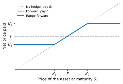
A long range forward, for a client who will buy the asset, is a long call with strike K_{2} and a short put with strike K_{1}. If the client buys the asset in the market at S_{T} and settles the options, the net price paid is S_{T} - \max(S_{T} - K_{2}, 0) + \max(K_{1} - S_{T}, 0) = \min(\max(S_{T}, K_{1}), K_{2}), that is, S_{T} inside the band, K_{2} above it and K_{1} below it. The client is protected against prices above K_{2} and pays for that protection by giving up the savings when the price falls below K_{1}. The strikes are usually chosen so that the put sold pays for the call bought, making the contract zero cost. As the band narrows around the forward price, the range forward becomes a plain forward.

Figure 1 compares the price paid under a range forward with the price paid without a hedge and under a forward.

Figure 1: Net price paid at maturity by a buyer of the asset under a long range forward with strikes K_{1} < F < K_{2}, compared with buying at the market price S_{T} and with a forward at F.

A short range forward, for a client who will sell the asset, is the opposite position: a long put with strike K_{1} and a short call with strike K_{2}. The price received is again S_{T} clipped to the band [K_{1}, K_{2}].

Since a range forward is a portfolio of European options, its value is the value of its parts. A long range forward is worth C(K_{2}) - P(K_{1}), both priced with Black-Scholes. A positive value is paid by the client to the dealer up front, and a negative value by the dealer to the client. A zero-cost range forward fixes one strike and solves for the other so that C(K_{2}) = P(K_{1}), which takes trial and error or a spreadsheet rather than a formula. Since a call and a put struck at the forward price have the same value, C(F) = P(F), the zero-cost band always contains the forward price: K_{1} < F < K_{2}.

Example 1 An asset trades at $100, pays a dividend yield of 2%, and has a volatility of 25%. The risk-free rate is 5%. A client buys a one-year range forward with K_{1} = \$90 and K_{2} = \$115. The forward price is F = 100 e^{(0.05 - 0.02) \times 1} = \$103.05.

For the call with strike 115 and the put with strike 90, \begin{gathered} d_{1} = \frac{\ln(100/115) + (0.05 - 0.02 + 0.5 \times 0.25^{2}) \times 1}{0.25} = -0.3140, \qquad d_{2} = -0.5640, \\ C = 100 e^{-0.02} \operatorname{Φ}(-0.3140) - 115 e^{-0.05} \operatorname{Φ}(-0.5640) = \$5.60, \\ d_{1} = \frac{\ln(100/90) + (0.05 - 0.02 + 0.5 \times 0.25^{2}) \times 1}{0.25} = 0.6664, \qquad d_{2} = 0.4164, \\ P = 90 e^{-0.05} \operatorname{Φ}(-0.4164) - 100 e^{-0.02} \operatorname{Φ}(-0.6664) = \$4.23. \end{gathered} The range forward is worth 5.603 - 4.227 = \$1.38, which the client pays up front. Keeping K_{1} = \$90, the client pays nothing when K_{2} = \$120.68, the strike at which the call is worth $4.23.

Variations of the Black-Scholes Framework

Binary Options

Binary options pay either a certain amount of cash or units of a risky asset if the underlying asset is above or below a certain strike price. For example, a cash-or-nothing call could pay Q if the stock price is above the strike price K or nothing otherwise. An asset-or-nothing call could pay 1 unit of the stock if the stock price is above the strike K or nothing otherwise.

Figure 2: Payoffs at maturity of a cash-or-nothing call that pays Q and an asset-or-nothing call that pays one share, both with strike K.

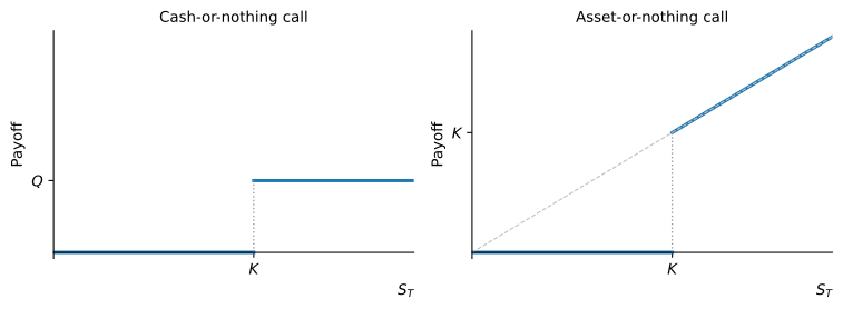
Interestingly, a European call option can be seen as a long asset-or-nothing call and a short cash-or-nothing call. Indeed, a European call pays S - K if S > K at maturity, which can be seen as receiving S and paying K whenever S > K, implying that C = \underbrace{S e^{-\delta T} \operatorname{Φ}(d_{1})}_{\text{asset-or-nothing call}} - \underbrace{K e^{-r T} \operatorname{Φ}(d_{2})}_{\text{cash-or-nothing call}}

Similarly, a European put can be seen as a long cash-or-nothing put and a short asset-or-nothing put: P = \underbrace{K e^{-r T} \operatorname{Φ}(-d_{2})}_{\text{cash-or-nothing put}} - \underbrace{S e^{-\delta T} \operatorname{Φ}(-d_{1})}_{\text{asset-or-nothing put}}

The following table shows the prices of asset-or-nothing options that pay 1 share of the stock, and cash-or-nothing options that pay Q, whenever the option is ITM at maturity.

Type	Call	Put
Asset-or-nothing	S e^{-\delta T} \operatorname{Φ}(d_{1})	S e^{-\delta T} \operatorname{Φ}(-d_{1})
Cash-or-nothing	Q e^{-r T} \operatorname{Φ}(d_{2})	Q e^{-r T} \operatorname{Φ}(-d_{2})

Example 2 Consider a stock that pays a dividend yield of 3% and that has a volatility of returns of 35%. The stock price is $150 and the risk-free rate is 8%.

First, let’s price an asset-or-nothing call that pays 1 share of the stock if the stock price in 6 months is above $150. We can then compute d_{1} = \frac{\ln(150/150) + (0.08 - 0.03 + 0.5 \times 0.35^{2}) \times 0.5}{0.35 \sqrt{0.5}} = 0.2248

The cost of the asset-or-nothing call is 150 e^{-0.03 \times 0.5} \operatorname{Φ}(0.2248) = \$87.02. The price of an otherwise equivalent asset-or-nothing put is 150 e^{-0.03 \times 0.5} \operatorname{Φ}(-0.2248) = \$60.74.

Example 3 Using the data in Example 2, consider a cash-or-nothing call that pays $100 if the stock price in 6 months is above $150. We can compute d_{2} = d_{1} - 0.35 \sqrt{0.5} = -0.0227

The cost of the cash-or-nothing call is then 100 e^{-0.08 \times 0.5} \operatorname{Φ}(-0.0227) = \$47.17. The cost of an otherwise equivalent cash-or-nothing put is 100 e^{-0.08 \times 0.5} \operatorname{Φ}(0.0227) = \$48.91.

Gap Options

A gap option uses different strike prices to determine when and how much to pay. For example, a gap call pays S_{T} - K_{1} when S_{T} > K_{2}, and zero otherwise. Here K_{2} determines if the option is ITM at expiration whereas K_{1} determines how much the option pays if it is ITM. A gap call is equivalent to a standard European call when K_{1} = K_{2}.

The binary options above price it directly. When S_{T} > K_{2}, the gap call delivers one share and takes K_{1} in cash, so it is a long asset-or-nothing call and a short position in K_{1} cash-or-nothing calls that pay $1, both triggered at K_{2}. Hence, \text{Gap Call} = S e^{-\delta T} \operatorname{Φ}(d_{1}) - K_{1} e^{-r T} \operatorname{Φ}(d_{2}), where d_{1} = \frac{\ln(S/K_{2}) + (r - \delta + 0.5 \sigma^{2}) T}{\sigma \sqrt{T}}, \qquad d_{2} = d_{1} - \sigma \sqrt{T}. The trigger K_{2} enters d_{1} and d_{2} because it decides when the binaries pay, while K_{1} only scales the cash leg.

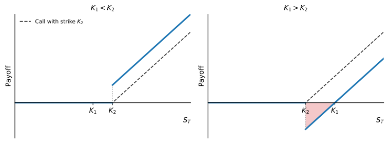
Unlike a standard call, a gap call can have a negative payoff. When K_{1} > K_{2} and S_{T} ends between K_{2} and K_{1}, the option is triggered and the holder pays K_{1} - S_{T}. Its price can therefore be zero or even negative. For a given trigger K_{2}, the gap call costs nothing when the cash leg equals the asset leg, that is, when K_{1} = S e^{(r - \delta) T} \operatorname{Φ}(d_{1}) / \operatorname{Φ}(d_{2}).

Figure 3 compares the two cases with a standard call struck at the trigger.

Figure 3: Payoffs at maturity of a gap call that pays S_{T} - K_{1} when S_{T} > K_{2}, compared with a standard call with strike K_{2}. The shaded area marks the negative payoffs when K_{1} > K_{2}.

Example 4 Suppose you want to price an option that pays S_{T} - 180 if S_{T} > 220 in 10 months. The option is written on a non-dividend paying asset whose current price is $200 and that has a volatility of returns of 40%. The risk-free rate is 6% per year with continuous compounding.

The option in the example is a gap call option where K_{1} = 180 and K_{2} = 220. This implies, d_{1} = \frac{\ln(200/220) + (0.06 + 0.5 (0.40)^{2}) (10/12)}{0.40 \sqrt{10/12}} = 0.0585, \qquad d_{2} = d_{1} - 0.40 \sqrt{10/12} = -0.3067. The gap call price is then given by, \text{Gap Call} = 200 \operatorname{Φ}(0.0585) - 180 e^{-0.06 \times 10/12} \operatorname{Φ}(-0.3067) = \$39.68

A gap put pays K_{1} - S_{T} when S_{T} < K_{2}, and zero otherwise. It is a long position in K_{1} cash-or-nothing puts and a short asset-or-nothing put, both triggered at K_{2}, so its price is \text{Gap Put} = K_{1} e^{-r T} \operatorname{Φ}(-d_{2}) - S e^{-\delta T} \operatorname{Φ}(-d_{1})

Example 5 Using the data in Example 4, the price of a gap put is \text{Gap Put} = 180 e^{-0.06 \times 10/12} \operatorname{Φ}(0.3067) - 200 \operatorname{Φ}(-0.0585) = \$10.90

Forward Start Options

A forward start option is a European call or put that starts at a future time \tau and expires at time T > \tau. They are typically implicit in employee stock option plans, and are often structured so that the strike price equals the asset price at time \tau, that is, K = S_{\tau}.

Because the strike is set equal to the stock price at \tau, the ratio S_{\tau}/K = S_{\tau}/S_{\tau} = 1, so \ln(S_{\tau}/K) = 0. This means d_{1} and d_{2} are deterministic at time 0: they do not depend on the realized value of S_{\tau}. The value of the option at time \tau is therefore: \begin{aligned} C_{\tau} & = S_{\tau} e^{-\delta (T - \tau)} \operatorname{Φ}(d_{1}) - S_{\tau} e^{-r (T - \tau)} \operatorname{Φ}(d_{2}) \\ P_{\tau} & = S_{\tau} e^{-r (T - \tau)} \operatorname{Φ}(-d_{2}) - S_{\tau} e^{-\delta (T - \tau)} \operatorname{Φ}(-d_{1}) \end{aligned} where d_{1} = \frac{(r - \delta + 0.5 \sigma^{2}) (T - \tau)}{\sigma \sqrt{T - \tau}}, \qquad d_{2} = d_{1} - \sigma \sqrt{T - \tau}.

The price of the option today is then V = \operatorname{E}^{*}(V_{\tau}) e^{-r \tau} where the expectation is taken with respect to the risk-neutral measure.

Since the risk-neutral expected stock price is \operatorname{E}^{*}(S_{\tau}) = S e^{(r - \delta) \tau}, we have that \operatorname{E}^{*}(S_{\tau}) e^{-r \tau} = S e^{-\delta \tau}. Therefore: \begin{aligned} C & = \left(S e^{-\delta (T - \tau)} \operatorname{Φ}(d_{1}) - S e^{-r (T - \tau)} \operatorname{Φ}(d_{2})\right) e^{-\delta \tau} \\ P & = \left(S e^{-r (T - \tau)} \operatorname{Φ}(-d_{2}) - S e^{-\delta (T - \tau)} \operatorname{Φ}(-d_{1})\right) e^{-\delta \tau} \end{aligned} with the same d_{1} and d_{2}. We can then see that the value of a forward start option is e^{-\delta \tau} times the value of a similar option starting today.

Example 6 Consider a stock with S = \$100, r = 10\%, \delta = 4\%, and \sigma = 30\%. Price an at-the-money forward start call that starts at \tau = 6 months and expires at T = 12 months.

The option has a time span of T - \tau = 6 months. Since \ln(S_\tau/K) = 0 at the start date, the d values depend only on this span: d_{1} = \frac{(0.10 - 0.04 + 0.5 \times 0.09) \times 0.5}{0.30 \sqrt{0.5}} = 0.2475, \qquad d_{2} = 0.2475 - 0.30 \sqrt{0.5} = 0.0354.

The forward start call is worth C = \left(100 e^{-0.04 \times 0.5} \operatorname{Φ}(0.2475) - 100 e^{-0.10 \times 0.5} \operatorname{Φ}(0.0354)\right) e^{-0.04 \times 0.5} = 9.69 \times 0.9802 = \$9.50

As expected, this equals e^{-\delta \tau} = e^{-0.02} = 0.9802 times the value of a standard at-the-money call with 6 months to maturity, which is \$9.69.

Forward start options can be packed together in what is known as a cliquet option, which consists of a series of call or put options with rules determining how the strike price is set.

For example, a cliquet might consist of 20 at-the-money three-month options. The total life would then be five years. When one option expires, a new at-the-money option comes into existence. This cliquet is therefore a portfolio of 20 forward starting options that can be valued using the formula above.

Chooser Options

A chooser option allows the buyer to choose at an intermediate time before expiration whether to get a European call or put option. If the chooser option starts at time 0 and matures at T, then at time \tau (0 < \tau < T) the buyer chooses whether it is a put or call with strike K and expiring at T.

As with forward start options, we first value the contract at \tau. At that date the buyer takes whichever option is more valuable, so the chooser is worth \max(C_{\tau}, P_{\tau}). Using the identity \max(C_{\tau}, P_{\tau}) = C_{\tau} + \max(P_{\tau} - C_{\tau}, 0) and put-call parity, P_{\tau} - C_{\tau} = K e^{-r (T - \tau)} - S_{\tau} e^{-\delta (T - \tau)} we get: \max(C_{\tau}, P_{\tau}) = C_{\tau} + \max\!\left(K e^{-r (T - \tau)} - S_{\tau} e^{-\delta (T - \tau)},\ 0\right) Factoring e^{-\delta(T-\tau)} out of the max gives: \max(C_{\tau}, P_{\tau}) = C_{\tau} + e^{-\delta (T - \tau)} \max\left(K e^{-(r - \delta)(T - \tau)} - S_{\tau}, 0\right)

This is the payoff of a call with strike K and expiring at T plus e^{-\delta (T - \tau)} puts with strike \widetilde{K} = K e^{-(r - \delta)(T - \tau)} and expiring at time \tau.

Example 7 Consider a stock with S = \$100, r = 8\%, \delta = 0\%, and \sigma = 30\%. Price a chooser option with strike K = \$100 and final maturity T = 1 year, where the choice is made at \tau = 0.5 years.

The chooser option is equivalent to a call with K = 100 and T = 1 year, plus e^{-\delta (T - \tau)} = e^{0} = 1 put with strike \widetilde{K} = 100 e^{-(0.08 - 0)(0.5)} = \$96.08 and maturity \tau = 0.5 years.

For the call: \begin{gathered} d_{1} = \frac{\ln(100/100) + (0.08 + 0.5 \times 0.09) \times 1}{0.30 \times 1} = 0.4167, \qquad d_{2} = 0.4167 - 0.30 = 0.1167, \\ C = 100 \operatorname{Φ}(0.4167) - 100 e^{-0.08} \operatorname{Φ}(0.1167) = \$15.71. \end{gathered} For the put with strike \widetilde{K} = 96.08 and maturity 0.5 years: \begin{gathered} d_{1} = \frac{\ln(100/96.08) + (0.08 + 0.5 \times 0.09) \times 0.5}{0.30 \sqrt{0.5}} = 0.4831, \qquad d_{2} = 0.4831 - 0.30 \sqrt{0.5} = 0.2710, \\ P = 96.08 e^{-0.08 \times 0.5} \operatorname{Φ}(-0.2710) - 100 \operatorname{Φ}(-0.4831) = \$4.85. \end{gathered} The chooser option costs 15.71 + 1 \times 4.85 = \$20.56.

Path-Dependent Options

The payoffs of some options might depend not only on the final value of the stock but on the full history of the stock price until maturity. These types of options are commonly called path-dependent options.

The closed-form prices above work because each payoff depends only on S_{T}, whose risk-neutral distribution is lognormal. When the payoff depends on the path, we need the distribution of the whole history. A binomial tree handles this directly, as long as we follow each path separately. The stock tree itself still recombines, since an up move followed by a down move leads to the same price as a down move followed by an up move. What does not recombine is the information the payoff needs: two paths that end at the same price can have different maxima or averages.

Following every path works for a few steps but not for many. A tree with n steps has only n + 1 final prices but 2^{n} paths, more than a million when n = 20. In practice, one either records at each node the extra piece of information the payoff needs, such as the running maximum or whether the barrier has been hit, or simulates many risk-neutral paths of the stock and averages their discounted payoffs.

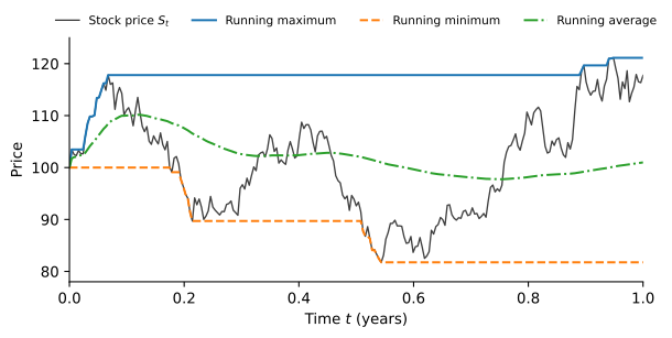
Figure 4 shows one simulated path of the stock with the running maximum, minimum and average that the options below use.

Figure 4: One simulated year of daily stock prices starting at S_{0} = 100 with \sigma = 0.30, together with the running maximum, running minimum, and running average of the path.

Lookback Options

The payoff of a lookback option depends on the maximum (S_{\textit{max}}) or minimum (S_{\textit{min}}) value of the stock until maturity. Both are taken over the whole life of the option, including the initial price S_{0}, and in a binomial tree over the nodes of each path. There are two types of lookback options, namely floating and fixed lookbacks.

A floating lookback call pays S_{T} - S_{\textit{min}} at time T. The idea is that the strike of the call is now replaced by the minimum price the stock reaches before maturity. Since by definition S_{\textit{min}} \leq S_{T}, we always have that the payoff of the floating lookback call is non-negative. Similarly, the payoff of a floating lookback put is defined as S_{\textit{max}} - S_{T} and by construction is also non-negative.

A fixed lookback call is like a regular call whose final payoff depends on the maximum value of the stock during the lifetime of the option, that is, it pays \max(S_{\textit{max}} - K, 0) at maturity. A fixed lookback put pays \max(K - S_{\textit{min}}, 0) at maturity.

The table below summarizes the payoffs of the different lookback options.

Type	Call	Put
Floating lookback	S_{T} - S_{\textit{min}}	S_{\textit{max}} - S_{T}
Fixed lookback	\max(S_{\textit{max}} - K, 0)	\max(K - S_{\textit{min}}, 0)

Asian Options

The payoff of an Asian option is related to the average stock price \bar{S} from time 0 until T. In continuous time this is defined as \bar{S}_{T} = \frac{1}{T} \int_{0}^{T} S_{t} dt In a binomial tree, the average is computed as the arithmetic mean of the stock price at each node along the path, including t = 0.

As with lookback options, there are two types of Asian options:

• An average price call pays \max(\bar{S}_{T} - K, 0) whereas an average price put pays \max(K - \bar{S}_{T}, 0) at maturity.
• An average strike call pays \max(S_{T} - \bar{S}_{T}, 0) whereas an average strike put pays \max(\bar{S}_{T} - S_{T}, 0).

Averaging smooths the path, so the average price is less volatile than the final price. An average price option is therefore usually cheaper than the corresponding European option, which makes it popular with firms that buy or sell a commodity or a currency regularly over a period and care about the average price they pay or receive.

There is no exact analytic valuation for Asian options based on the arithmetic average used here (options on the geometric average do have one), but they can be approximately valued by assuming that the average stock price is lognormally distributed.

Pricing on a Binomial Tree

Analytic formulas exist for lookback options, and Asian options can be approximated, but a binomial tree prices both directly. The next example prices a lookback and an Asian option on the same tree.

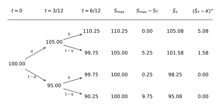
Example 8 Consider a non-dividend paying stock that trades for $100. Every 3 months, the stock price can increase or decrease by 5%. The risk-free rate is 6% per year with continuous compounding. We price two options that expire in 6 months: a floating lookback put that pays S_{\textit{max}} - S_{T}, and an average price call that pays \max(\bar{S}_{T} - K, 0) with K = 100.

Since both payoffs depend on the path, we draw the full tree for the stock with all four histories, and compute for each history its maximum, its average (including t = 0), and the two payoffs.

The risk-neutral probability of an up-move is q = \frac{e^{0.06 \times 3/12} - 0.95}{1.05 - 0.95} = 0.6511 Working backward through the tree, the lookback put L and the Asian call A are worth \begin{aligned} L_{u} & = (0 q + 5.25 (1 - q)) e^{-0.06 \times 3/12} = 1.80 \\ L_{d} & = (0.25 q + 9.75 (1 - q)) e^{-0.06 \times 3/12} = 3.51 \\ L & = (1.80 q + 3.51 (1 - q)) e^{-0.06 \times 3/12} = 2.36 \\[4pt] A_{u} & = (5.08 q + 1.58 (1 - q)) e^{-0.06 \times 3/12} = 3.80 \\ A_{d} & = (0 q + 0 (1 - q)) e^{-0.06 \times 3/12} = 0 \\ A & = (3.80 q + 0 (1 - q)) e^{-0.06 \times 3/12} = 2.44 \end{aligned} Alternatively, we could obtain both prices directly from the final payoffs: \begin{aligned} L & = (0 q^{2} + 5.25 q (1 - q) + 0.25 (1 - q) q + 9.75 (1 - q)^{2}) e^{-0.06 \times 6/12} = 2.36 \\ A & = (5.08 q^{2} + 1.58 q (1 - q) + 0 (1 - q) q + 0 (1 - q)^{2}) e^{-0.06 \times 6/12} = 2.44 \end{aligned}

Barrier Options

Barrier options are either call or put options that get activated or deactivated depending on whether the stock hits a barrier from above or below.

In options come into existence only if the stock price hits the barrier before option maturity. Out options die if the stock price hits the barrier before option maturity.

Up options require that the stock hits the barrier from below, whereas down options require that the stock hits the barrier from above.

Combining the two directions with in/out and call/put gives eight possible barrier options:

Direction	Type	Call	Put
Up	In	Up-and-in call	Up-and-in put
Up	Out	Up-and-out call	Up-and-out put
Down	In	Down-and-in call	Down-and-in put
Down	Out	Down-and-out call	Down-and-out put

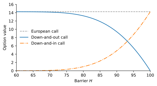
A key property of barrier options is that an in and out option with the same direction, strike, barrier, and maturity always sum to the corresponding plain European option. For example, a down-and-in call plus a down-and-out call (same parameters) equals a standard European call.

Figure 5 shows how the barrier moves value between the two calls. A barrier far below the stock price is rarely touched, so the down-and-out call is almost a European call. As H approaches S, the barrier is touched almost surely and the value shifts to the down-and-in call.

Figure 5: Black-Scholes prices of a one-year down-and-in and down-and-out call against the barrier H, with S = K = 100, r = 5\% and \sigma = 30\%. The two always add up to the European call, shown dashed.

Example 9 Consider a down-and-in call with barrier $90, strike price $110, and expiring in 6 months. The stock price is currently $100.

• Case 1: During the next six months, the stock goes down to $85 but then finishes at $120. The down-and-in call pays 120 - 110 = \$10.
• Case 2: During the next six months, the stock never goes below $90 and finishes at $140. The down-and-in call pays nothing since even though it is in-the-money it never gets activated.
• Case 3: During the next six months, the stock goes down to $85 and finishes at $105. Even though the down-and-in call gets activated, it is out-of-the-money at maturity and hence pays nothing.

Barrier options can be priced using a binomial tree by tracking, at each node, whether the barrier has been hit along that path. Analytical formulas also exist within the Black-Scholes framework for all eight standard combinations. Exercise 8 prices a down-and-in and a down-and-out call this way.

Two practical points matter for barrier options. First, the contract states how often the barrier is checked: continuously, or only at specified times such as daily closes. A barrier checked less often is hit less often, so a knock-out option with discrete monitoring is worth more than one with continuous monitoring, and a knock-in option is worth less. A binomial tree checks the barrier only at its nodes, so it behaves like a discretely monitored contract and needs many steps to price a continuously monitored one.

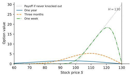
Second, barrier options are hard to hedge near the barrier. Close to the barrier of an up-and-out call, a small rise in the stock price can wipe out a large in-the-money payoff, so the option’s value falls steeply as the stock rises and its delta is large and negative. A cash-or-nothing option has the same problem near the strike as maturity approaches, since a small move decides whether it pays the full amount or nothing. A dealer who delta hedges these positions must trade large amounts of stock for small price moves.

Figure 6 shows the problem for an up-and-out call. Far from maturity, the chance of hitting the barrier keeps the option cheap everywhere. Close to maturity, the value approaches the call payoff up to the barrier and then drops to zero over a few dollars of stock price.

Figure 6: Black-Scholes prices of an up-and-out call with strike K = 100 and barrier H = 130 against the stock price, for three maturities, with r = 5\% and \sigma = 30\%. The dotted line is the payoff of a call that is never knocked out.

Other Exotic Options

The options below are beyond the scope of this course but are worth knowing about as they appear frequently in practice.

Compound Options

Options written on other options are known as compound options. We can then have four possible combinations:

• Call on call
• Put on call
• Call on put
• Put on put

These options arise naturally when analyzing the equity of a leveraged firm (equity is a call on the firm’s assets, and an option on the equity is therefore a compound option). They can be valued analytically using an extension of the Black-Scholes framework. Intuitively, the price of a compound option is quite low compared with the underlying option, since it gives the right to pay for the right to buy (or sell) the asset.

Exchange Options

An exchange option is an option to exchange one asset for another. For example, an option to exchange one unit of U for one unit of V. The payoff is then \max(V_{T} - U_{T}, 0).

Measuring prices in units of U turns the payoff into U_{T} \max(V_{T}/U_{T} - 1, 0), a call on the ratio V/U with a strike of 1. Two features of the Black-Scholes formula change. The interest rate drops out, since the holder pays with units of U, not with cash. The relevant volatility is that of the ratio V/U, which depends on how the two assets are correlated: two assets that move together have a stable ratio and make a cheap exchange option. A binomial tree for this option needs two dimensions, one for each asset, with the correlation built into the joint moves, and an analytical formula exists within the Black-Scholes framework.

Basket Options

A basket option is an option to buy or sell a portfolio of assets. This can be valued by calculating the first two moments of the value of the basket at option maturity and then assuming it is lognormal.

Shout Options

A shout option lets the buyer shout once during the life of the option, at a time \tau of their choice, and lock in the intrinsic value at that moment. A shout call then pays the larger of the usual payoff and the intrinsic value at the shout: \max(S_{T} - K, S_{\tau} - K) = \max(S_{T} - S_{\tau}, 0) + S_{\tau} - K The buyer gets the gain up to the shout plus a fresh at-the-money call from then on. The option resembles a lookback, since the buyer tries to shout near the maximum, but it is cheaper because the shout may not catch the maximum.

Non-Standard American Options

In practice, many American type options have restrictions about when they can be exercised. Some American options are exercisable only on specific dates (Bermudans), whereas other options can be exercised early only after a certain lock out period has elapsed.

Some American options have a strike price that changes over the life of the contract, such as warrants or convertibles.

Practice Problems

Problems 1 to 6 are based on an asset with the following characteristics:

Variable	Value
S	100
r	10%
\delta	4%
\sigma	30%

Problem 1 Compute the price of a long range forward with maturity 9 months, and strikes K_{1} = \$90 and K_{2} = \$120.

Solution

The long range forward is a long call with strike K_{2} and a short put with strike K_{1}. For the call, we have: \begin{gathered} d_{1} = \frac{\ln(100/120) + (0.10 - 0.04 + \frac{1}{2} 0.30^{2})(9/12)}{0.30 \sqrt{9/12}} = -0.3986, \qquad \operatorname{Φ}(d_{1}) = 0.3451, \\ d_{2} = -0.3986 - 0.30 \sqrt{9/12} = -0.6585, \qquad \operatorname{Φ}(d_{2}) = 0.2551, \\ C = 100 e^{-0.04 (9/12)} \times 0.3451 - 120 e^{-0.10 (9/12)} \times 0.2551 = \$5.09 \end{gathered} For the put we have: \begin{gathered} d_{1} = \frac{\ln(100/90) + (0.10 - 0.04 + \frac{1}{2} 0.30^{2}) (9/12)}{0.30 \sqrt{9/12}} = 0.7086, \qquad \operatorname{Φ}(-d_{1}) = 0.2393, \\ d_{2} = 0.7086 - 0.30 \sqrt{9/12} = 0.4488, \qquad \operatorname{Φ}(-d_{2}) = 0.3268, \\ P = 90 e^{-0.10 (9/12)} \times 0.3268 - 100 e^{-0.04 (9/12)} \times 0.2393 = \$4.06 \end{gathered} Therefore, the long range forward costs 5.09 - 4.06 = \$1.02.

Problem 2 Compute the price of a cash-or-nothing binary option with maturity 9 months that pays $50 whenever S_{T} > 100.

Solution

For the cash-or-nothing option we have: \begin{gathered} d_{1} = \frac{\ln(100/100) + (0.10 - 0.04 + \frac{1}{2} 0.30^{2}) (9/12)}{0.30 \sqrt{9/12}} = 0.3031, \qquad \operatorname{Φ}(d_{1}) = 0.6191, \\ d_{2} = 0.3031 - 0.30 \sqrt{9/12} = 0.0433, \qquad \operatorname{Φ}(d_{2}) = 0.5173 \end{gathered} Therefore, the cash-or-nothing costs 50 e^{-0.10 (9/12)} (0.5173) = \$23.99.

Problem 3 Compute the price of an asset-or-nothing binary option with maturity 9 months that pays one unit of the stock whenever S_{T} > 100.

Solution

For the asset-or-nothing option we have: \begin{gathered} d_{1} = \frac{\ln(100/100) + (0.10 - 0.04 + \frac{1}{2} 0.30^{2}) (9/12)}{0.30 \sqrt{9/12}} = 0.3031, \qquad \operatorname{Φ}(d_{1}) = 0.6191 \end{gathered} Therefore, the asset-or-nothing is worth 100 e^{-0.04 (9/12)} (0.6191) = \$60.08.

Problem 4 Compute the price of a gap put option with maturity 9 months, that pays 90 - S_{T} whenever S_{T} < 110.

Solution

We have that: \begin{gathered} d_{1} = \frac{\ln(100/110) + (0.10 - 0.04 + \frac{1}{2} 0.30^{2}) (9/12)}{0.30 \sqrt{9/12}} = -0.0637, \qquad \operatorname{Φ}(-d_{1}) = 0.5254, \\ d_{2} = -0.0637 - 0.30 \sqrt{9/12} = -0.3235, \qquad \operatorname{Φ}(-d_{2}) = 0.6269 \end{gathered} Therefore, the gap put should cost 90 e^{-0.10 (9/12)} (0.6269) - 100 e^{-0.04 (9/12)} (0.5254) = \$1.35.

Problem 5 Compute the price of a forward start put option that starts in 9 months, with final maturity in 15 months, and that is struck at-the-money when it starts.

Solution

The difference between the final maturity and the starting date is 6 months, hence: \begin{gathered} d_{1} = \frac{(0.10 - 0.04 + \frac{1}{2} 0.30^{2}) (6/12)}{0.30 \sqrt{6/12}} = 0.2475, \qquad \operatorname{Φ}(-d_{1}) = 0.4023, \\ d_{2} = 0.2475 - 0.30 \sqrt{6/12} = 0.0354, \qquad \operatorname{Φ}(-d_{2}) = 0.4859 \end{gathered} Therefore, the forward start put should cost \left( 100 e^{-0.10 \times 6/12} \times 0.4859 - 100 e^{-0.04 \times 6/12} \times 0.4023 \right) e^{-0.04 \times 9/12} = \$6.59.

Problem 6 Compute the price of a chooser option with maturity 15 months, strike K = \$110, and where the buyer can choose whether it is a call or a put in 6 months.

Solution

The chooser option is equivalent to a call with strike 110 and maturity 15 months, plus e^{-0.04 (15 - 6)/12} = 0.9704 puts with strike 110 e^{-(0.10 - 0.04)(15 - 6)/12} = \$105.16 and maturity 6 months. To compute the price of the call: \begin{gathered} d_{1} = \frac{\ln(100/110) + (0.10 - 0.04 + \frac{1}{2} 0.30^{2}) (15/12)}{0.30 \sqrt{15/12}} = 0.1072, \qquad \operatorname{Φ}(d_{1}) = 0.5427, \\ d_{2} = 0.1072 - 0.30 \sqrt{15/12} = -0.2283, \qquad \operatorname{Φ}(d_{2}) = 0.4097, \\ C = 100 e^{-0.04 (15/12)} (0.5427) - 110 e^{-0.10 (15/12)} (0.4097) = \$11.85 \end{gathered} To compute the price of the put: \begin{gathered} d_{1} = \frac{\ln(100/105.16) + (0.10 - 0.04 + \frac{1}{2} 0.30^{2}) (6/12)}{0.30 \sqrt{6/12}} = 0.0103, \qquad \operatorname{Φ}(-d_{1}) = 0.4959, \\ d_{2} = 0.0103 - 0.30 \sqrt{6/12} = -0.2018, \qquad \operatorname{Φ}(-d_{2}) = 0.5800, \\ P = 105.16 e^{-0.10 (6/12)} (0.5800) - 100 e^{-0.04 (6/12)} (0.4959) = \$9.41 \end{gathered} Therefore, the chooser option is worth 11.85 + 0.9704 (9.41) = \$20.98.

Problem 7 Consider a non-dividend paying stock that trades for $100. Every 3 months, the stock price can increase or decrease by 10%. The risk-free rate is 10% per year with continuous compounding. Compute the price of the following path-dependent options expiring in 6 months:

1. A floating lookback put that pays S_{\textit{max}} - S_{T} at maturity.
2. A fixed lookback call that pays \max(S_{\textit{max}} - 100, 0) at maturity.
3. An average price Asian call option that pays \max(\bar{S} - 100, 0) at maturity.
4. A floating lookback call that pays S_{T} - S_{\textit{min}} at maturity.

Solution

To price these options we need to compute the maximum, minimum and average price per path. The stock tree recombines, but paths 2 and 3 end at the same price with different maxima, minima and averages, so we specify the payoffs for each path.

Path	t = 0	t = 0.25	t = 0.5
1	100	110	121
2	100	110	99
3	100	90	99
4	100	90	81

The risk-neutral probability of the stock going up each period is q = \frac{e^{0.10 \times 3/12} - 0.9}{1.1 - 0.9} = 0.6266.

The risk-neutral probability of the stock price going up twice is q^{2} = 0.3926, whereas the risk-neutral probability of the stock price going up and then down, or down and then up is q (1 - q) = 0.2340. Finally, the risk-neutral probability of the stock price going down twice is (1 - q)^{2} = 0.1394.

1. The possible payoffs at maturity of the floating lookback put are:

   Path	S_{\textit{max}}	S_{\textit{max}} - S_{T}
   1	121	0
   2	110	11
   3	100	1
   4	100	19

   Therefore, the price of the floating lookback put is \left( 0 q^{2} + 11 q (1 - q) + 1 (1 - q) q + 19 (1 - q)^{2} \right) e^{-0.10 \times 6/12} = \$5.19.

2. The possible payoffs at maturity of the fixed lookback call are:

   Path	S_{\textit{max}}	\max(S_{\textit{max}} - 100, 0)
   1	121	21
   2	110	10
   3	100	0
   4	100	0

   Therefore, the price of the fixed lookback call is \left( 21 q^{2} + 10 q (1 - q) + 0 (1 - q) q + 0 (1 - q)^{2} \right) e^{-0.10 \times 6/12} = \$10.07.

3. The possible payoffs at maturity of the average price Asian call are:

   Path	\bar{S}	\max(\bar{S} - 100, 0)
   1	110.33	10.33
   2	103	3
   3	96.33	0
   4	90.33	0

   Therefore, the price of the average price Asian call is \left( 10.33 q^{2} + 3 q (1 - q) + 0 (1 - q) q + 0 (1 - q)^{2} \right) e^{-0.10 \times 6/12} = \$4.53.

4. The possible payoffs at maturity of the floating lookback call are:

   Path	S_{\textit{min}}	S_{T} - S_{\textit{min}}
   1	100	21
   2	99	0
   3	90	9
   4	81	0

   Therefore, the price of the floating lookback call is \left( 21 q^{2} + 0 q (1 - q) + 9 (1 - q) q + 0 (1 - q)^{2} \right) e^{-0.10 \times 6/12} = \$9.85.

Problem 8 Consider a non-dividend paying stock that trades for $100. Every 3 months, the stock price can increase or decrease by 10%. The risk-free rate is 10% per year with continuous compounding. Using a 2-step binomial tree, compute the price of the following barrier options expiring in 6 months with strike price K = \$95 and barrier H = \$90:

1. A down-and-in call that pays \max(S_{T} - 95, 0) at maturity, provided the stock touched $90 or below at some point before maturity.
2. A down-and-out call that pays \max(S_{T} - 95, 0) at maturity, provided the stock never touched $90 or below before maturity.
3. Verify that the sum of the down-and-in and down-and-out call prices equals the price of an otherwise equivalent European call.

Solution

Using the same tree as in Exercise 7, the four paths and their terminal stock prices are:

Path	t = 0	t = 0.25	t = 0.5	Barrier hit?	\max(S_{T} - 95, 0)
1	100	110	121	No	26
2	100	110	99	No	4
3	100	90	99	Yes	4
4	100	90	81	Yes	0

Paths 2 and 3 end at the same price with the same payoff, but only path 3 touched the barrier. The risk-neutral probability of an up-move is q = 0.6266 (from Exercise 7).

1. The down-and-in call activates only on paths 3 and 4. Path 4 ends out of the money, so only path 3 pays: \text{Down-and-in call} = 4 (1 - q) q e^{-0.10 \times 6/12} = \$0.89.

2. The down-and-out call pays only on paths 1 and 2, which never hit the barrier: \text{Down-and-out call} = \left(26 q^{2} + 4 q (1 - q)\right) e^{-0.10 \times 6/12} = \$10.60.

3. The standard European call pays on paths 1, 2 and 3. Its price is C = \left(26 q^{2} + 4 q (1 - q) + 4 (1 - q) q\right) e^{-0.10 \times 6/12} = \$11.49. Indeed, 0.89 + 10.60 = \$11.49: path 3 pays through the down-and-in call, paths 1 and 2 through the down-and-out call, and together they pay exactly what the European call pays on every path.