Forward and Futures Markets
Forward Contracts
A forward contract is an agreement to buy or sell an asset at a future date for a price fixed today, called the delivery price, which we denote by K. The party that agrees to buy has a long position, and the party that agrees to sell has a short position. If the price of the asset at maturity is S_{T}, then the payoff of the long position is S_{T} - K.
Suppose the asset price at maturity is greater than the delivery price. In that case, we purchase the asset for K and immediately sell it for S_{T}, generating a payoff of S_{T} - K. If, on the other hand, S_{T} < K, then the payoff is negative since under the terms of the contract we are required to purchase the asset for K which we can only sell at a lower price S_{T}.
Figure 1 plots the payoff of a long forward as a function of the price of the asset at maturity S_{T}. The payoff increases in S_{T} and cuts the x-axis at the delivery price K.
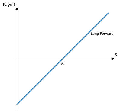
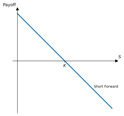
Figure 2 shows the payoff of a short forward position, given by K - S_{T}. The short forward payoff is then the mirror image with respect to the x-axis of the long forward position. By fixing the price at K, the seller is happy when prices go down but is unhappy when prices increase.
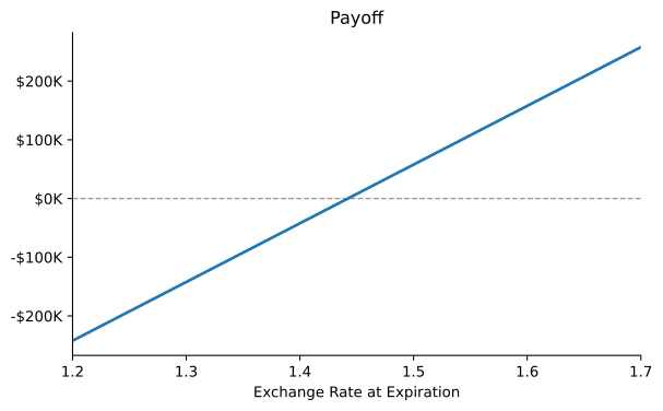
Example 1 (Payoff from buying currency forward) On May 24, 2010, the treasurer of a corporation entered into a long forward contract to buy £1 million in six months at an exchange rate of $1.4422 per pound sterling. The agreement binds the corporation to pay $1,442,200 for £1 million on November 24, 2010. What are the possible outcomes?
We can compute the contract payoff for different exchange rate values six months from now, giving us an idea of the possible outcomes depending on the exchange rate in six months.
| Exchange Rate | 1.2000 | 1.3000 | 1.4000 | 1.5000 | 1.6000 |
|---|---|---|---|---|---|
| Payoff | -242,200 | -142,200 | -42,200 | 57,800 | 157,800 |
The figure below plots the payoff of this long forward contract as a function of the currency exchange rate at maturity.
When a new forward contract is entered, nobody pays anything up front, so the delivery price must be set to make the contract worth zero to both parties. The delivery price with that property is the forward price F. At inception, then, K = F. Later, the forward price for the same delivery date moves with the market while K stays fixed, and the contract acquires a positive value for one party and a negative value for the other. What determines F is the subject of Forward and Futures Prices.
Forwards trade over-the-counter (OTC): traders working for buy-side firms, such as fund managers and corporate treasurers, contact sell-side firms, such as large international banks, directly. The terms can be negotiated to fit the needs of a client, and the contract is usually settled in full at maturity. Each party is therefore exposed to the risk that the other defaults before then.
Futures Contracts
A futures contract is a forward contract traded on an organized exchange such as the Chicago Mercantile Exchange (CME) or the Chicago Board Options Exchange (CBOE). Futures are written on a wide variety of asset classes such as physical commodities, equity indices, foreign currencies, interest rates and even abstract quantities such as volatility. The exchange standardizes the terms of the contract, such as the size, the expiration dates, the delivery method and the quality of the good, so that all contracts with the same expiration are interchangeable. Standardization concentrates liquidity: Working (1953) shows that the cost of hedging explains why trading in a commodity concentrates in a single exchange and contract, and why hedgers often accept a “poor” hedge if it is cheaper.
Example 2 These are examples of some futures contracts:
- Buy 100 oz. of gold at $1,400 per oz. in December
- Sell £62,500 at $1.2620 per £ in June
- Sell 1,000 barrels of oil at $70 per barrel in July
Traditionally, all futures traded on physical trading floors organized into segmented areas called pits. Traders and floor brokers interacted directly with each other in face-to-face transactions, in a system commonly known as open-outcry. With the advent of technology and later on the COVID-19 pandemic, almost all futures trading today occurs electronically.
Electronic trading is usually implemented by recording bids and offers in an electronic limit-order book. A limit order that cannot execute immediately, because the bid is lower than the best offer or the offer is higher than the best bid, is recorded in the book. These orders can be cancelled at no cost, otherwise they usually stay active until the end of that day’s trading session. Market orders, on the other hand, execute immediately at the best bid or offer available when the order is received.
Futures trade for longer hours than stocks. For example, the E-mini S&P 500 (ES) trades Sunday through Friday from 5 p.m. to 4 p.m. Central Time (CT), with a one-hour break each day.
Margin and Daily Settlement
What makes a futures contract different from a forward is how gains and losses are paid. Each day, the exchange determines a settlement price for every contract, and every position is marked to market: the change in the settlement price from the previous day, times the contract size, is credited to the margin accounts of the winning side and debited from those of the losing side. In effect, the contract is rewritten every day at the new settlement price. A trader who buys at a futures price F_{0} accumulates gains and losses that add up by expiration to S_{T} - F_{0}, the payoff of a forward with delivery price F_{0}, paid in daily installments.
To trade futures, a trader deposits cash or marketable securities in a margin account with a broker. The account must stay above a maintenance margin, and if losses take it below that level, the trader receives a margin call and must deposit more funds or the position is closed. The exchange sets margins from the risk of the position, based on how far the price can move in a day, so the margin per contract rises with both the contract size and the volatility of the price. The exchange’s clearinghouse becomes the buyer to every seller and the seller to every buyer, and because losses are collected every day, a default can only cost it about one day’s price move. Futures traders, unlike forward counterparties, do not need to worry about who is on the other side of their trades.
Example 3 (Margin account on the E-mini S&P 500) The E-mini S&P 500 futures contract is one of the most liquid futures in the world. The contract value is $50 \times the futures price.
Say you deposit $12,000 in your margin account and buy one E-mini futures at 4,645.00. The next day the futures price settles at 4,656.75, a gain of 11.75 index points with respect to the previous settlement, so your account is credited 50 \times 11.75 = \$587.50 and rises to $12,587.50. If the day after the futures price settles at 4,652.25, your account loses 50 \times 4.50 = \$225.00, bringing it down to $12,362.50. The table below continues for one more day.
| Day | Futures Price | Gain/Loss | Margin Account |
|---|---|---|---|
| 0 | 4,645.00 | 12,000.00 | |
| 1 | 4,656.75 | 587.50 | 12,587.50 |
| 2 | 4,652.25 | -225.00 | 12,362.50 |
| 3 | 4,658.50 | 312.50 | 12,675.00 |
Over the three days the futures price rose 13.50 points, and the account gained 50 \times 13.50 = \$675, the same as a forward entered at 4,645.00 and closed at 4,658.50.
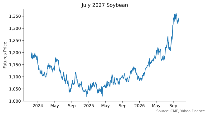
The settlement price is what is usually reported as the price of the contract for that day. Figure 3 plots the settlement price of the July 2027 soybean futures contract since it started trading.
Settlement and Delivery
A futures contract that is still open at expiration is settled in one of two ways. For many commodity contracts, the final settlement involves the physical delivery of the underlying good, so the contract specifications must state the size, quality, and delivery locations of the commodity that can be delivered.
Other contracts are cash settled: the final payment is the contract size times the value of a reference index. Equity index futures are settled this way, because delivering every stock in the index in the right proportions would be cumbersome and most likely impossible. Short-term interest rate futures, such as SOFR futures, are also cash settled. Treasury note and bond futures, by contrast, are settled by delivering Treasury securities.
All futures contracts have an expiration date, and for a given underlying asset there are usually several expirations trading at any given point in time.
Almost nobody who trades futures intends to make or take delivery. Traders close their positions before expiration, or roll them into the next contract by selling the expiring contract and buying a later one, and every gain or loss along the way is settled in cash through the margin account. For them, a physically settled contract works exactly like a cash-settled one. Delivery matters only to the few commercial firms with the storage and transport to handle the physical good, and only in the last days of a contract. A trader who keeps a long position into delivery without a place to store the commodity is in serious trouble, as the case of negative oil prices in Forward and Futures Prices shows.
Open Interest
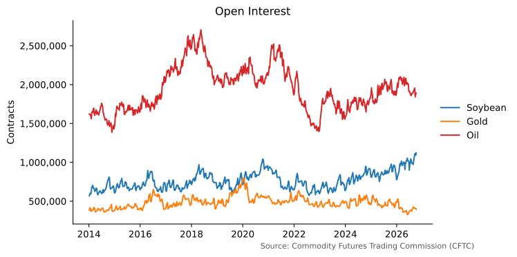
Exchanges also report the total number of contracts outstanding, called the open interest. For every long position there is a corresponding short position, so the open interest measures the total number of long positions, or equivalently the total number of short positions, open at any given point in time. Figure 4 displays the evolution of the open interest for all soybean, gold and oil futures starting Jan-2014.
A large open interest could reflect strong demand for short positions, long positions, or both. The Commodity Futures Trading Commission (CFTC) publishes detailed weekly information about open interest for all futures in their Commitments of Traders (COT) Reports. The reports separate commercial traders, mostly hedgers, from noncommercial traders, mostly speculators, and they are the source of the evidence on hedging pressure in Futures Prices vs. Expected Future Spot Prices.
The Spot Price
Futures of different maturities on the same underlying trade side by side on one exchange under the same contract terms, and holding any of them requires no storage and no capital beyond margin. No-arbitrage therefore always applies among futures contracts. Whether it also ties them to the cash market depends on how easily traders can arbitrage the difference between the cash price and the futures price, called the basis.
For a stock index, the basis is easy to arbitrage. Traders can buy or short the basket of stocks in the S&P 500 and hold it at a known cost, so index arbitrage keeps the E-mini futures close to the cash index, as Forward and Futures Prices shows. The same holds for individual stocks and freely convertible currencies, and for these assets the cash price is the spot price.
Physical commodities are different. They come in different grades and locations, and moving or storing them takes time and money. Brent and West Texas Intermediate are both crude oil, but they are different oils delivered in different places, and they trade at different prices. Even gold, the same metal everywhere, is a different asset in London than in New York: if it could be teleported, the two would have the same price, but moving bars takes time and money. What trades around the clock in London is not metal but unallocated gold, a claim on a bank rather than bars in a vault. Buying a particular lot and delivering it against a futures contract carries risk, so the basis of a commodity is not held in place by arbitrage.
What a commodity trader can buy and sell at a known cost is its futures contract, standardized in grade, size, and location. For this reason, we define the spot price of a commodity as the price of the closest-to-maturity futures contract, the nearby contract. It is the price traders hedge against and the price against which contracts of other maturities are quoted. The spot price can be far from the cash price of the physical good, and that gap is not a pricing error. When analyzing commodity futures we therefore take the nearby futures, not the physical commodity, as the underlying asset.
More formally, if we denote by F(t, T) the futures price at time t of a contract expiring at time T, the spot price is defined as S_{t} = F(t, T_{1}), where T_{1} is the nearest expiration date after t.
The figure below plots the cotton spot price since 2018 and the July 2027 cotton futures contract since it started trading.
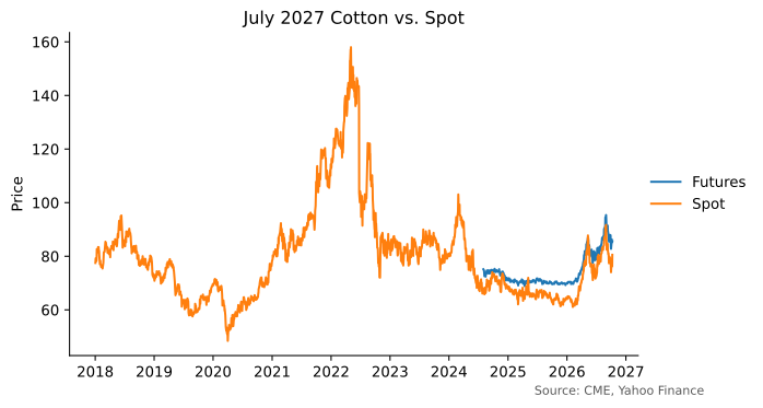
The gap between the two lines is the spread between the July contract and the nearby contract. Once the July contract becomes the nearby contract, the two lines coincide by definition. Note also that the spot series switches contracts at every expiration, so it can jump on roll dates even when no contract price moved. Its day-to-day changes are not the returns of any position someone held.
Hedging the Basis
If arbitrage does not hold the basis of a commodity in place, someone must bear its risk. That someone is mostly the merchants and processors who buy, store, and sell the physical good. A grain merchant who buys wheat and stores it for a few months is exposed to the price of wheat. Selling futures removes most of that exposure, and what is left is the basis. Working (1953) argues that this is the point of the trade. The merchant buys wheat because its cash price is low relative to the futures price and expects the gap to change in their favor. Hedging, in his words, “is not properly comparable with insurance. It is a sort of arbitrage.”
Working, Holbrook. 1953. “Futures Trading and Hedging.” American Economic Review 43 (3): 314–43.
Denote by P_{t} the cash price of the merchant’s wheat and by F_{t} the price of the futures contract used to hedge it, so that the basis is B_{t} = P_{t} - F_{t}. A merchant who buys one bushel at time 0, sells one futures, and unwinds both at time 1 gains (P_{1} - P_{0}) - (F_{1} - F_{0}) = B_{1} - B_{0}. \tag{1} The price level drops out, and only the change in the basis remains. The example below uses Working’s prices for wheat at Kansas City in the 1951-52 crop year.
Example 4 (Hedging wheat in storage) On September 4, 1951, a merchant buys No. 2 Hard Winter wheat in Kansas City at 232.50 cents per bushel and sells the December wheat futures at 238.25 cents, a basis of -5.75 cents. On December 1, the merchant sells the wheat at 252 cents and buys back the December futures at 252 cents, a basis of zero.
| Sep 4 | Dec 1 | Gain | |
|---|---|---|---|
| Cash wheat (long) | 232.50 | 252.00 | 19.50 |
| December futures (short) | 238.25 | 252.00 | -13.75 |
| Basis | -5.75 | 0.00 | 5.75 |
The merchant earns 5.75 cents per bushel for storing the wheat for three months, exactly what the basis promised on September 4. The wheat was the grade delivered on the December futures, so the two prices had to converge as the contract expired. Unhedged, the gain would have been 19.50 cents, but a fall in wheat prices would have turned it into a loss. With the hedge, the merchant is paid for storage, not for a bet on the price of wheat.
The basis also tells the merchant when not to store. On May 1, 1952, wheat of the same grade sold at a premium of 18 cents over the July futures, because old-crop wheat was scarce and the new crop would arrive in large volume by July. The premium was a signal to sell stocks, not to carry them. A merchant who carried hedged wheat from May 1 to July 1 lost 24.50 cents per bushel as the premium fell to a discount, a loss as sure, Working writes, as that on Christmas trees held until December 26. The basis pays for storage when stocks are plentiful and charges for it when they are scarce, the pattern behind the price of storage in Forward and Futures Prices.
The hedge in Example 4 was nearly riskless because the merchant’s wheat was the grade the contract delivers and the hedge was lifted in the delivery month. Most hedges are not so clean. The merchant’s wheat may differ in grade or location from what the contract delivers, or the hedge may be lifted long before the contract expires. Cash and futures prices then do not move one for one, the basis is risky, and one futures per unit of the cash commodity is not always the hedge that removes the most risk. Johnson (1960) and Stein (1961) treat the cash and futures holdings as a portfolio chosen for its mean and variance. If the merchant sells h futures per unit of the cash commodity, the gain per unit is (P_{1} - P_{0}) - h (F_{1} - F_{0}), and Johnson (1960) shows that its variance is smallest at h^{*} = \frac{\operatorname{Cov}(P_{1} - P_{0}, F_{1} - F_{0})}{\operatorname{V}(F_{1} - F_{0})}, \tag{2} the slope of a regression of changes in the cash price on changes in the futures price. This hedge removes a fraction \rho^{2} of the variance of the unhedged position, where \rho is the correlation between the two price changes. Ederington (1979) estimates h^{*} for Treasury bill, mortgage-backed (GNMA), wheat, and corn futures. He finds it significantly different from one in most cases, usually below one, and finds that hedges held for four weeks remove more risk than hedges held for two.
Johnson, Leland L. 1960. “The Theory of Hedging and Speculation in Commodity Futures.” Review of Economic Studies 27 (3): 139–51.
Stein, Jerome L. 1961. “The Simultaneous Determination of Spot and Futures Prices.” American Economic Review 51 (5): 1012–25.
Ederington, Louis H. 1979. “The Hedging Performance of the New Futures Markets.” Journal of Finance 34 (1): 157–70.
Anderson, Ronald W., and Jean-Pierre Danthine. 1981. “Cross Hedging.” Journal of Political Economy 89 (6): 1182–96.
The minimum-variance hedge ignores expected profits. Anderson and Danthine (1981) show that a merchant holding q units of the cash commodity and maximizing \operatorname{E}[\pi] - \frac{\lambda}{2} \operatorname{V}(\pi), where \pi is profit and \lambda measures risk aversion, sells N_{F} = h^{*} q + \frac{F_{0} - \operatorname{E}[F_{1}]}{\lambda \operatorname{V}(F_{1} - F_{0})} \tag{3} futures. The first term is the risk-minimizing hedge. The second is a pure speculation, the position a speculator with the same views and risk aversion would take: a merchant who expects the futures price to fall sells more than the hedge, and one who expects it to rise sells less. Working’s merchant has no view on the price level, so the second term is zero, and sells one futures per unit of wheat, N_{F} = q. The merchant’s view on the basis enters instead through q, the amount of wheat to store (Anderson and Danthine 1981). Pure risk minimization and Working’s arbitrage are two special cases of one portfolio problem (Ederington 1979).
The speculative term is also where the risk premium of Futures Prices vs. Expected Future Spot Prices enters. If hedgers are net short and speculators must be paid to take the long side, the futures price is below its expected value, \operatorname{E}[F_{1}] > F_{0}, and the second term is negative: the hedger sells fewer futures than the pure hedge. The premium is the cost of hedging, and a hedger who pays it buys less of it.
SOFR Futures
The London Inter-Bank Offered Rate in US dollars, or LIBOR USD, was for half a century the reference rate for corporate loans denominated in USD. LIBOR was also quoted in other major currencies such as the Japanese Yen (JPY) or the Swiss Franc (CHF). After the LIBOR manipulation cases that came to light in 2012, and with unsecured interbank borrowing too thin to anchor the rate, regulators set out to replace LIBOR (Duffie and Stein 2015).
Duffie, Darrell, and Jeremy C. Stein. 2015. “Reforming LIBOR and Other Financial Market Benchmarks.” Journal of Economic Perspectives 29 (2): 191–212.
In 2014, the Federal Reserve Board and the New York Fed convened the Alternative Reference Rates Committee (ARRC), a group of private-market participants tasked with identifying robust alternatives to USD LIBOR and supporting a transition away from LIBOR. In 2017, the ARRC selected the Secured Overnight Financing Rate (SOFR) as the replacement for LIBOR USD.
SOFR is the rate on overnight loans of cash collateralized by Treasury securities, that is, on Treasury repurchase transactions (repos). Because the loans are secured and the market is deep, SOFR is close to a risk-free rate, unlike LIBOR, which measured banks’ unsecured borrowing cost. Since SOFR is an overnight rate while loans and swaps need rates over months, an active SOFR futures market has developed in which traders hedge and lock in the average of SOFR over future periods. SOFR futures are cash settled against realized SOFR rates. For 1-month SOFR futures the reference index is an arithmetic average whereas for 3-month SOFR futures the reference index is a geometric average of SOFR rates.
The notional value of the 3-month SOFR futures is equal to $2,500 \times the contract grade IMM index, which is computed as 100 minus the business-day compounded SOFR per annum during the contract reference quarter. For 1-month SOFR futures, the index is computed similarly but against an arithmetic average of SOFR during the contract delivery month.
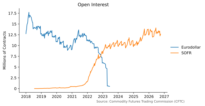
The new contract has been a success. In April 2023 CME converted the remaining open interest in Eurodollar futures and options, the LIBOR contracts, into SOFR contracts (Mondo Visione 2023). By 2025, SOFR futures and options traded a record 5.4 million contracts a day, more than a third of all interest rate trading at CME (CME Group 2026), and on August 13, 2025 open interest in SOFR futures reached a record 13.7 million contracts (CME Group 2025). Figure 6 shows the transition in open interest.
Mondo Visione. 2023. CME Group Completes Key Milestones in Conversion of Eurodollar Futures and Options. Mondo Visione, April 2023. https://mondovisione.com/media-and-resources/news/cme-group-completes-key-milestones-in-conversion-of-eurodollar-futures-options-2023424/.
CME Group. 2026. CME Group Reports Record Annual ADV of 28.1 Million Contracts in 2025, up 6% Year over Year. CME Group press release, January 5, 2026. https://www.cmegroup.com/media-room/press-releases/2026/1/05/cme_group_reportsrecordannualadvof281millioncontractsin2025up6ye.html.
CME Group. 2025. CME Group Interest Rate Futures Open Interest Sets New Record of 40 Million Contracts. CME Group press release, August 14, 2025. https://www.cmegroup.com/media-room/press-releases/2025/8/14/cme_group_interestratefuturesopeninterestsetsnewrecordof40millio.html.
Practice Problems
Problem 1 A forward contract is defined as:
- The right but not the obligation to purchase or sell an asset in the future at a given fixed price for a given quantity.
- A commitment to purchase or sell an asset at a given fixed price for a given quantity.
- An asset that pays a fixed amount at maturity.
- A physical position in the underlying asset.
Solution
A forward contract is a commitment to purchase or sell an asset at a given fixed price for a given quantity. The answer is b.Problem 2 Imagine that you agree to purchase 1 million euros in 9 months from now at an exchange rate of $1.12 per euro. What would be your payoff if the exchange rate in 9 months is $1.02 per euro?
Solution
The payoff is computed as 1{,}000{,}000 \times (1.02 - 1.12) = -\$100{,}000.Problem 3 Consider an E-mini S&P 500 futures contract. Remember that the contract value is defined as $50 times the futures price. Yesterday’s futures price settlement was 4,296.12, whereas today, the S&P 500 futures price settled at 4,175.20. Compute the change in a trader’s margin account if she bought one futures yesterday.
Solution
The change will be 50 \times (4{,}175.20 - 4{,}296.12) = -\$6{,}046.Problem 4 A merchant buys 50,000 bushels of corn at $4.10 per bushel and hedges by selling March corn futures at $4.35. Two months later the merchant sells the corn at $4.42 and buys back the futures at $4.55. Each corn futures contract is for 5,000 bushels.
- What is the basis when the hedge is placed and when it is lifted, and what is the merchant’s gain per bushel?
- The standard deviation of two-month changes in the cash price is $0.20, that of the futures price is $0.25, and the correlation between the two is 0.9. How many futures contracts minimize the variance of the hedged position, and what fraction of the unhedged variance do they remove?
Solution
- The basis is 4.10 - 4.35 = -\$0.25 when the hedge is placed and 4.42 - 4.55 = -\$0.13 when it is lifted. The corn gains 4.42 - 4.10 = \$0.32 and the short futures loses 4.55 - 4.35 = \$0.20, so the merchant gains $0.12 per bushel, the change in the basis.
- The minimum-variance hedge ratio is h^{*} = 0.9 \times 0.20 / 0.25 = 0.72, so the merchant sells 0.72 \times 50{,}000 / 5{,}000 = 7.2, or about 7 contracts. The hedge removes \rho^{2} = 0.81, or 81%, of the unhedged variance.