Class 12

The Risk-Neutral Measure

A stock that pays no dividends over [0, T] and a money-market account follow \frac{\mathop{}\!\mathrm{d}S}{S} = \mu \mathop{}\!\mathrm{d}t+ \sigma \mathop{}\!\mathrm{d}B, \qquad \frac{\mathop{}\!\mathrm{d}\beta}{\beta} = r \mathop{}\!\mathrm{d}t, \qquad \frac{\mathop{}\!\mathrm{d}\Lambda}{\Lambda} = -r \mathop{}\!\mathrm{d}t- \lambda \mathop{}\!\mathrm{d}B, where only the part of the SDF \Lambda correlated with the stock matters for pricing it. The pricing equation makes \lambda = (\mu - r) / \sigma the stock’s Sharpe ratio. The process \mathcal{E} = \Lambda \beta satisfies \mathop{}\!\mathrm{d}\mathcal{E} / \mathcal{E} = -\lambda \mathop{}\!\mathrm{d}B, so it is a positive (local) martingale, and when it is a true martingale it defines the risk-neutral measure \mathop{}\!\mathrm{d}\operatorname{P}^{*} / \mathop{}\!\mathrm{d}\operatorname{P}= \mathcal{E}_{T} / \mathcal{E}_{0}. By Girsanov’s theorem, \mathop{}\!\mathrm{d}B^{*} = \mathop{}\!\mathrm{d}B+ \lambda \mathop{}\!\mathrm{d}t is a \operatorname{P}^{*}-Brownian motion, and \frac{\mathop{}\!\mathrm{d}S}{S} = r \mathop{}\!\mathrm{d}t+ \sigma \mathop{}\!\mathrm{d}B^{*}. \tag{1} Every asset V driven by the same B has the same Sharpe ratio, so \mathop{}\!\mathrm{d}V / V = r \mathop{}\!\mathrm{d}t+ \sigma_{V} \mathop{}\!\mathrm{d}B^{*}: under \operatorname{P}^{*} all assets earn the risk-free rate. Since \Lambda V is a martingale, V_{0} = \operatorname{E}\left(\frac{\Lambda_{T}}{\Lambda_{0}} V_{T}\right) = \operatorname{E}^{*}\left(e^{-\int_{0}^{T} r_{s} \mathop{}\!\mathrm{d}s} V_{T}\right). \tag{2} Prices are expected payoffs discounted at the risk-free rate, provided the expectation uses \operatorname{P}^{*}.

Bonds, Futures, and Forwards

A zero-coupon bond has V_{T} = 1, so P(T) = \operatorname{E}^{*}(e^{-\int_{0}^{T} r_{s} \mathop{}\!\mathrm{d}s}). A futures position costs nothing to enter and pays its gains \mathop{}\!\mathrm{d}F continuously, so \operatorname{E}(\Lambda \mathop{}\!\mathrm{d}F) = 0, or \operatorname{E}^{*}(\mathop{}\!\mathrm{d}F) = 0: the futures price is a \operatorname{P}^{*}-martingale, and F(T) = \operatorname{E}^{*}(S_{T}). The forward price \varphi(T) gives the forward contract zero value, which yields \varphi(T) = F(T) + \frac{\operatorname{Cov}^{*}\left(e^{-\int_{0}^{T} r_{s} \mathop{}\!\mathrm{d}s}, S_{T}\right)}{P(T)}. \tag{3} Forward and futures prices coincide when this covariance is zero, in particular when r is constant.

The Black-Scholes Formula

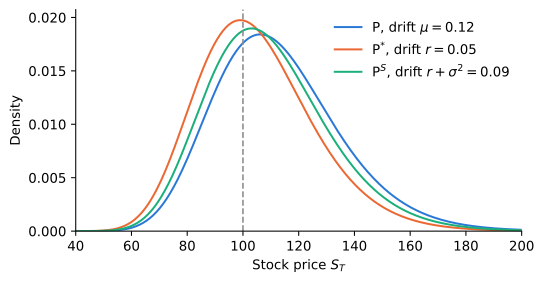
With constant parameters, (1) gives S_{T} = S_{0} e^{(r - \frac{1}{2} \sigma^{2}) T + \sigma B^{*}_{T}}, so \ln S_{T} is normal under \operatorname{P}^{*} with mean \ln S_{0} + (r - \frac{1}{2} \sigma^{2}) T and variance \sigma^{2} T. Splitting the call payoff into S_{T} \mathbf{1}_{\{S_{T} > K\}} - K \mathbf{1}_{\{S_{T} > K\}}, C_{0} = S_{0} \operatorname{P}^{S}(S_{T} > K) - K e^{-r T} \operatorname{P}^{*}(S_{T} > K), \tag{4} where \operatorname{P}^{S} is the measure with density \Lambda_{T} S_{T} / (\Lambda_{0} S_{0}), which uses the stock as the unit of account (a change of numeraire). Under \operatorname{P}^{S} the stock has expected return r + \sigma^{2}, so only the drift differs across the three measures, as Figure 1 shows. Evaluating both probabilities, C = S_{0} N(d_{1}) - K e^{-r T} N(d_{2}), \qquad P = K e^{-r T} N(-d_{2}) - S_{0} N(-d_{1}), \tag{5} with d_{1} = \frac{\ln(S_{0} / K) + \left(r + \frac{1}{2} \sigma^{2}\right) T}{\sigma \sqrt{T}}, \qquad d_{2} = d_{1} - \sigma \sqrt{T}, and N(d) the standard normal CDF. Here N(d_{2}) is the risk-neutral probability that the call is exercised. The expected return \mu never appears. Subtracting the two prices gives put-call parity, C - P = S_{0} - K e^{-r T}, which holds in any model.

Figure 1: Density of the stock price S_{T} after one year under the three measures, with S_{0} = 100, \sigma = 0.20, \mu = 0.12, and r = 0.05. The volatility is the same under all three; only the drift changes. The dashed line marks a strike of 100.

The Black-Scholes PDE

If V(S, t) is the price of a derivative paying f(S_{T}), Itô’s lemma under (1) gives its drift, and that drift must equal r V: r S \frac{\partial V}{\partial S} + \frac{1}{2} \sigma^{2} S^{2} \frac{\partial^{2} V}{\partial S^{2}} + \frac{\partial V}{\partial t} = r V, \qquad V(S, T) = f(S). \tag{6} All derivatives on S solve the same equation and differ only in the terminal condition. The diffusion term \sigma S \, \partial V / \partial S shows that holding the derivative and selling \partial V / \partial S shares (its delta) removes all exposure to \mathop{}\!\mathrm{d}B, which was the original argument of Black and Scholes. The solution of (6) is the expectation (2), the Feynman-Kac formula.

The Merton Model

Real prices gap. Let N be a Poisson process with intensity \lambda (from here on, \lambda is a jump intensity) and Y_{i} iid \mathcal{N}(m, s^{2}) log jump sizes, independent of B. In the model of Merton, S_{t} = S_{0} \exp\left(\left(\mu - \tfrac{1}{2} \sigma^{2} - \lambda k\right) t + \sigma B_{t} + \sum_{i = 1}^{N_{t}} Y_{i}\right), \qquad k = \operatorname{E}(e^{Y}) - 1 = e^{m + \frac{1}{2} s^{2}} - 1. \tag{7} Each jump multiplies the price by e^{Y_{i}}, and k is the expected percentage jump. The -\lambda k correction keeps \operatorname{E}(S_{t}) = S_{0} e^{\mu t}. Given N_{t} = n, the log return is normal, so its density is a Poisson mixture of normals. Every cumulant beyond the variance comes from the jumps: \kappa_{2} = \sigma^{2} t + \lambda t (m^{2} + s^{2}), \qquad \kappa_{3} = \lambda t \left(m^{3} + 3 m s^{2}\right), \qquad \kappa_{4} = \lambda t \left(m^{4} + 6 m^{2} s^{2} + 3 s^{4}\right). \tag{8} With m < 0 the skewness \kappa_{3} / \kappa_{2}^{3/2} is negative and the excess kurtosis \kappa_{4} / \kappa_{2}^{2} is positive. They shrink like 1 / \sqrt{t} and 1 / t, so jumps matter most over short horizons.

Itô’s Formula with Jumps and Changes of Intensity

Compensated jumps. If the Z_{i} are iid and independent of N, then \sum_{i \leq N_{t}} Z_{i} - \lambda \operatorname{E}(Z) t is a martingale. A process with jumps is a martingale when its continuous drift plus \lambda times its expected jump is zero.

Itô’s formula. For X_{t} = X_{0} + \int a_{s} \mathop{}\!\mathrm{d}s + \int b_{s} \mathop{}\!\mathrm{d}B_{s} + \sum_{i \leq N_{t}} Z_{i} and f twice continuously differentiable, \mathop{}\!\mathrm{d}f(X_{t}) = \left(a f'(X_{t}) + \tfrac{1}{2} b^{2} f''(X_{t})\right) \mathop{}\!\mathrm{d}t+ b f'(X_{t}) \mathop{}\!\mathrm{d}B_{t} + \left(f(X_{t-} + \Delta X_{t}) - f(X_{t-})\right). \tag{9} The jump term is the exact change in f, not a Taylor expansion. Applied to (7), \mathop{}\!\mathrm{d}S_{t} / S_{t-} = (\mu - \lambda k) \mathop{}\!\mathrm{d}t+ \sigma \mathop{}\!\mathrm{d}B_{t} + (e^{Y} - 1) \mathop{}\!\mathrm{d}N_{t}, whose jump term has compensator \lambda k \mathop{}\!\mathrm{d}t.

Changing the intensity. For \lambda^{*} > 0, the positive martingale Z_{t} = \left(\frac{\lambda^{*}}{\lambda}\right)^{N_{t}} e^{-(\lambda^{*} - \lambda) t} \tag{10} defines a measure under which N is Poisson with intensity \lambda^{*}. Brownian reweighting only shifts a drift, but the quadratic variation of N is random, so reweighting paths can change how often jumps occur. Jump sizes can be reweighted too.

Credit Spreads

A firm defaults at the first event of N, and bondholders lose a fraction L at default. If the SDF jumps by the factor 1 + \eta at default, \Lambda_{t} = e^{-r t} (1 + \eta)^{N_{t}} e^{-\lambda \eta t}, then \Lambda \beta is the density (10) with \lambda^{*} = \lambda (1 + \eta), and a bond priced e^{-c (T - t)} before default has spread c - r = \lambda^{*} L = (1 + \eta) \lambda L. \tag{11} With \eta > 0, defaults hit in bad times, and the spread exceeds the expected loss rate \lambda L.

Option Pricing with Jumps

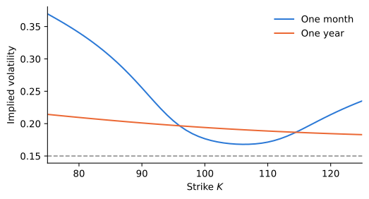
A stock position hedges \mathop{}\!\mathrm{d}B but not a jump of random size, because an option’s value changes nonlinearly in the jump. The market is incomplete: many risk-neutral measures price the stock, each with \mathop{}\!\mathrm{d}S_{t} / S_{t-} = (r - \lambda^{*} k^{*}) \mathop{}\!\mathrm{d}t+ \sigma \mathop{}\!\mathrm{d}B^{*}_{t} + (e^{Y} - 1) \mathop{}\!\mathrm{d}N_{t}. Merton assumed that jump risk is diversifiable and unpriced, so \lambda and the jump distribution are the same under \operatorname{P} and \operatorname{P}^{*}. The call price is then a Poisson mixture of Black-Scholes prices, C = \sum_{n = 0}^{\infty} e^{-\lambda' T} \frac{(\lambda' T)^{n}}{n!} \, C^{BS}(S_{0}, K, r_{n}, \sigma_{n}, T), \tag{12} with \lambda' = \lambda (1 + k), \sigma_{n}^{2} = \sigma^{2} + n s^{2} / T, and r_{n} = r - \lambda k + n \ln(1 + k) / T. Downward jumps raise the implied volatility of low strikes, producing the skew of Figure 2, which is steepest at short maturities.

For models without a formula like (12), (4) still holds, and both probabilities come from the risk-neutral characteristic function \phi of \ln S_{T} by the inversion formula \operatorname{P}(X > x) = \frac{1}{2} + \frac{1}{\pi} \int_{0}^{\infty} \operatorname{Im}(e^{-i u x} \phi(u)) / u \mathop{}\!\mathrm{d}u, using \phi^{S}(u) = \phi(u - i) / \phi(-i) for \operatorname{P}^{S}.

Figure 2: Black-Scholes implied volatility of Merton call prices against the strike for one-month and one-year options, with S_{0} = 100, r = 0.05, \sigma = 0.15, \lambda = 1, m = -0.08, and s = 0.10. The dashed line is the diffusion volatility.

Practice Problems

1. A stock follows \mathop{}\!\mathrm{d}S/ S = \mu \mathop{}\!\mathrm{d}t+ \sigma \mathop{}\!\mathrm{d}B with \mu = 0.10 and \sigma = 0.20, its price today is S_{0} = 100, and the risk-free rate is a constant r = 0.04.

   1. Compute \lambda and write the dynamics of S under \operatorname{P}^{*}.
   2. Another asset is driven by the same Brownian motion and has volatility \sigma_{V} = 0.50. What is its expected return under \operatorname{P}? Under \operatorname{P}^{*}?
   3. Compute the two-year futures price and the two-year forward price. Why are they equal?
   4. A log contract pays \ln S_{T} at T = 2. Use (2) to compute its price today.

2. A pension fund holds a stock index at S_{0} = 100 and buys a one-year European put with strike K = 95 as insurance. The index volatility is \sigma = 0.25 and r = 0.04. Use N(0.49) = 0.6879 and N(0.24) = 0.5948.

   1. Compute d_{1} and d_{2}, and the risk-neutral probability that the put is exercised.
   2. The put’s payoff is a long position in a contract paying K if S_{T} < K and a short position in a contract paying S_{T} if S_{T} < K. Price each contract using (4) and its analog for the put, and compute the put price.
   3. Use put-call parity to price the call with the same strike, and check it with (5).

3. A firm defaults with historical intensity \lambda = 0.02 per year, bondholders lose L = 0.5 at default, and r = 0.04. Its bonds trade at a credit spread of 300 basis points.

   1. Compute the expected loss rate, the risk-neutral intensity \lambda^{*}, and the jump \eta in the SDF at default.
   2. Compute the price of a five-year zero-coupon bond with face value 1 before default, and compare it with a risk-free bond.
   3. Compute the probability that the firm defaults within five years under \operatorname{P} and under \operatorname{P}^{*}.
   4. Evaluate the density Z_{5} in (10) on paths with no default and on paths with exactly one default by year five. Explain why default paths receive more weight under \operatorname{P}^{*}.