Class 2

Densities and Distribution Functions

A continuous random variable X has a density f(x) \geq 0 that integrates to one, and probabilities are areas under it, \operatorname{P}(a < X \leq b) = \int_{a}^{b} f(x) \, dx = F(b) - F(a), where F(x) = \operatorname{P}(X \leq x) is the CDF, with F'(x) = f(x). The density is not a probability: it can exceed one, and any single value has probability zero. The right tail, or survival function, is \operatorname{P}(X > x) = 1 - F(x). Sums become integrals, so \operatorname{E}(g(X)) = \int g(x) f(x) \, dx, and everything we did with discrete random variables carries over.

If Y = g(X) with g strictly increasing, then \operatorname{P}(Y \leq y) = \operatorname{P}(X \leq g^{-1}(y)), and differentiating gives f_{Y}(y) = f_{X}(g^{-1}(y)) \, \frac{d g^{-1}(y)}{d y}. \tag{1} The derivative accounts for how the transformation stretches or compresses intervals.

Uniform and Exponential

The uniform distribution on [a, b] has constant density 1 / (b - a), mean (a + b) / 2 and variance (b - a)^{2} / 12. It drives simulation through the inverse transform method: if F is continuous and strictly increasing and U \sim \text{Uniform}(0, 1), then X = F^{-1}(U) has CDF F.

The exponential distribution T \sim \text{Exp}(\lambda) models the waiting time for an event that occurs at a constant rate \lambda, such as a default with constant intensity, f(t) = \lambda e^{-\lambda t}, \qquad \operatorname{P}(T > t) = e^{-\lambda t}, \qquad \operatorname{E}(T) = \frac{1}{\lambda}, \qquad \operatorname{V}(T) = \frac{1}{\lambda^{2}}. Solving u = 1 - e^{-\lambda t} gives the simulation recipe T = -\ln(U) / \lambda.

The Gamma Distribution

The exponential distribution describes the waiting time for one event. The gamma distribution describes, among other things, the waiting time for several. Its density involves the gamma function \Gamma(\alpha) = \int_{0}^{\infty} x^{\alpha - 1} e^{-x} \mathop{}\!\mathrm{d}x, \qquad \alpha > 0. \tag{2} Integrating by parts gives \Gamma(\alpha + 1) = \alpha \Gamma(\alpha), and since \Gamma(1) = 1, \Gamma(n) = (n - 1)! for every positive integer n: the gamma function extends the factorial to non-integer arguments. We will also need \Gamma(1/2) = \sqrt{\pi}.

A random variable X \sim \text{Gamma}(\alpha, \lambda), with shape \alpha > 0 and rate \lambda > 0, has density f(x) = \frac{\lambda^{\alpha}}{\Gamma(\alpha)} x^{\alpha - 1} e^{-\lambda x}, \qquad x > 0. The substitution u = \lambda x in (2) shows that it integrates to one. For k \geq 1, the integrand of \operatorname{E}(X^{k}) is proportional to a gamma density with shape \alpha + k, so \operatorname{E}(X^{k}) = \frac{\Gamma(\alpha + k)}{\Gamma(\alpha) \lambda^{k}}, \qquad \operatorname{E}(X) = \frac{\alpha}{\lambda}, \qquad \operatorname{V}(X) = \frac{\alpha}{\lambda^{2}}. \tag{3} For \alpha \leq 1 the density decreases from its value at zero, while for \alpha > 1 it rises from zero to a peak at (\alpha - 1) / \lambda and then decays. With \alpha = 1 the gamma is the exponential distribution. A sum of n independent \text{Exp}(\lambda) waiting times is \text{Gamma}(n, \lambda), so the time of the n-th event in a Poisson process is gamma distributed.

The Normal Distribution

X \sim \mathcal{N}(\mu, \sigma^{2}) has density e^{-(x - \mu)^{2} / (2 \sigma^{2})} / \sqrt{2 \pi \sigma^{2}}, mean \mu and variance \sigma^{2}. Every normal probability reduces to the standard normal CDF \mathop{\Phi} through the Z-score, \operatorname{P}(X \leq x) = \mathop{\Phi}\left(\frac{x - \mu}{\sigma}\right), \qquad \mathop{\Phi}(-z) = 1 - \mathop{\Phi}(z). \tag{4} With z_{\alpha} defined by \operatorname{P}(Z > z_{\alpha}) = \alpha (z_{0.05} = 1.64, z_{0.025} = 1.96, z_{0.005} = 2.58), the (1 - \alpha) probability interval of X is [\mu - z_{\alpha/2} \sigma, \mu + z_{\alpha/2} \sigma]. It says where X is likely to fall; it is not a confidence interval.

If Z \sim \mathcal{N}(0, 1), then Z^{2} \sim \text{Gamma}(1/2, 1/2), the chi-squared distribution with one degree of freedom, so \operatorname{E}(Z^{2}) = 1, \operatorname{V}(Z^{2}) = 2 and \operatorname{E}(Z^{4}) = 3. A sum of k independent squared standard normals is chi-squared with k degrees of freedom, \text{Gamma}(k/2, 1/2), with mean k and variance 2 k.

The Lognormal Distribution

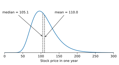
If X \sim \mathcal{N}(\mu, \sigma^{2}), then Y = e^{X} is lognormal: positive, skewed to the right, and the standard model for a stock price. Here \mu and \sigma^{2} are the mean and variance of \ln(Y), not of Y. Probabilities come from the logarithm, \operatorname{P}(Y \leq y) = \mathop{\Phi}((\ln(y) - \mu) / \sigma), and the moments are \operatorname{E}(Y^{\alpha}) = e^{\alpha \mu + \frac{1}{2} \alpha^{2} \sigma^{2}}, \qquad \operatorname{E}(Y) = e^{\mu + \frac{1}{2} \sigma^{2}}, \qquad \operatorname{SD}(Y) = \operatorname{E}(Y) \sqrt{e^{\sigma^{2}} - 1}. \tag{5} The median is e^{\mu}, below the mean, because the long right tail pulls the mean up (Figure 1). The (1 - \alpha) probability interval [e^{\mu - z_{\alpha/2} \sigma}, e^{\mu + z_{\alpha/2} \sigma}] divides and multiplies the median by the same factor, so it is not symmetric.

Figure 1: Density of a stock price in one year, Y = 100 e^{X} with X \sim \mathcal{N}(0.05, 0.30^{2}). The median 100 e^{0.05} lies below the mean 100 e^{0.05 + 0.045}.

The Bivariate Normal Distribution

Correlated normal returns are built from independent standard normals Z_{1} and Z_{2}, X = \mu_{X} + \sigma_{X} Z_{1}, \qquad Y = \mu_{Y} + \sigma_{Y} \left(\rho Z_{1} + \sqrt{1 - \rho^{2}} \, Z_{2}\right), \tag{6} which gives \operatorname{Cov}(X, Y) = \rho \sigma_{X} \sigma_{Y}. Three properties follow from the construction.

1. Linear combinations. a X + b Y is normal with mean a \mu_{X} + b \mu_{Y} and variance a^{2} \sigma_{X}^{2} + b^{2} \sigma_{Y}^{2} + 2 a b \rho \sigma_{X} \sigma_{Y}.
2. Conditional distribution. Given X = x, Y is normal with mean \mu_{Y} + \rho (\sigma_{Y} / \sigma_{X}) (x - \mu_{X}) and variance \sigma_{Y}^{2} (1 - \rho^{2}). The conditional mean is the regression line, with slope \operatorname{Cov}(X, Y) / \operatorname{V}(X).
3. Independence. X and Y are independent if and only if \rho = 0. This is special to jointly normal variables.

Heavy Tails

Daily returns have far more extreme moves than the normal distribution predicts. The Student t distribution with \nu degrees of freedom, T = Z / \sqrt{V / \nu} with V chi-squared and independent of Z, is normal given a random scale. Its density decays like the power |t|^{-(\nu + 1)}, so \operatorname{E}(|T|^{k}) is finite only for k < \nu, the variance \nu / (\nu - 2) requires \nu > 2, and \operatorname{E}(e^{\theta T}) = \infty for every \theta \neq 0. As \nu \to \infty it approaches the standard normal.

Practice Problems

1. The recovery rate R on a defaulted bond, per dollar of face value, is uniformly distributed on [0.2, 0.6].

   1. Compute \operatorname{E}(R) and \operatorname{SD}(R), and the probability that R > 0.5.
   2. A contract pays \max(R - 0.3, 0) per dollar of face value. Compute its expected payoff.
   3. A computer generates the uniform draws u = 0.10 and u = 0.75. Use the inverse transform method to turn them into simulated recovery rates.

2. The time W, in minutes, until the second trade in an illiquid bond has a \text{Gamma}(2, \lambda) distribution with \lambda = 2 per minute.

   1. Compute \operatorname{E}(W), \operatorname{SD}(W) and the value at which the density of W peaks.
   2. Integrate the density by parts to show that \operatorname{P}(W \leq t) = 1 - e^{-\lambda t} (1 + \lambda t), and compute \operatorname{P}(W \leq 1).
   3. Let D = 60 W be the same waiting time measured in seconds. Use (1) to find its density f_D, and show that D is again gamma distributed. Which parameter changes, and why?

3. The daily return of a $10 million portfolio is normal with mean 0.0004 and standard deviation 0.015.

   1. What is the probability that the portfolio loses more than 2% in a day?
   2. Using z_{0.05} = 1.64, find the dollar loss that is exceeded on only 5% of days.
   3. A risk manager estimates the daily variance with \hat{\sigma}^{2} = \frac{1}{21} \sum_{t = 1}^{21} (R_{t} - \mu)^{2}, using 21 independent daily returns R_{t} and the true mean \mu. Use the chi-squared distribution to compute \operatorname{E}(\hat{\sigma}^{2}) and the ratio \operatorname{SD}(\hat{\sigma}^{2}) / \sigma^{2}.

4. A stock trades at S_{0} = 50. Its log return over the year is \mathcal{N}(\mu, \sigma^{2}) with \mu = 0.06 and \sigma = 0.30.

   1. What is the probability that a call option with strike 60 and one year to maturity finishes in the money, that is, \operatorname{P}(S_{1} > 60)?
   2. Compute \operatorname{E}(S_{1}) and compare it with the median price S_{0} e^{\mu}.