Class 1
Probability Spaces and Random Variables
A discrete probability space (\Omega, \operatorname{P}) is a finite or countably infinite set of outcomes \Omega together with probabilities \operatorname{P}(\omega) \geq 0 that add up to one. An event is a subset A \subset \Omega, and its probability is \operatorname{P}(A) = \sum_{\omega \in A} \operatorname{P}(\omega). Unions, intersections and complements of events translate “or”, “and” and “not”. If A and B are disjoint, \operatorname{P}(A \cup B) = \operatorname{P}(A) + \operatorname{P}(B), and in particular \operatorname{P}(A^{C}) = 1 - \operatorname{P}(A).
A random variable X assigns a real number X(\omega) to each outcome. Its expectation and variance are \operatorname{E}(X) = \sum_{\omega \in \Omega} X(\omega) \operatorname{P}(\omega), \qquad \operatorname{V}(X) = \operatorname{E}\left((X - \operatorname{E}(X))^{2}\right) = \operatorname{E}(X^{2}) - \operatorname{E}(X)^{2}, and the covariance and correlation of X and Y are \operatorname{Cov}(X, Y) = \operatorname{E}(X Y) - \operatorname{E}(X) \operatorname{E}(Y), \qquad \rho_{X, Y} = \frac{\operatorname{Cov}(X, Y)}{\sigma_{X} \sigma_{Y}} \in [-1, 1].
Linear Combinations
For Z = \alpha X + \beta Y, expectations are linear while variances pick up the covariance: \operatorname{E}(Z) = \alpha \operatorname{E}(X) + \beta \operatorname{E}(Y), \qquad \operatorname{V}(Z) = \alpha^{2} \operatorname{V}(X) + \beta^{2} \operatorname{V}(Y) + 2 \alpha \beta \operatorname{Cov}(X, Y). \tag{1} If X_{1}, \ldots, X_{n} are uncorrelated with common variance \sigma^{2}, the sum has variance n \sigma^{2} and the average has variance \sigma^{2} / n. A sum of n shocks therefore drifts a distance of order \sqrt{n}, the scaling that will turn a random walk into Brownian motion.
Joint and Marginal Distributions
The probability mass function (pmf) of X is p_{X}(x) = \operatorname{P}(X = x), so that \operatorname{E}(X) = \sum_{x} x \, p_{X}(x). The joint pmf p_{X, Y}(x, y) = \operatorname{P}(X = x, Y = y) contains everything about X and Y. Summing over one variable recovers the other’s pmf, p_{X}(x) = \sum_{y} p_{X, Y}(x, y), \qquad p_{Y}(y) = \sum_{x} p_{X, Y}(x, y), and expectations of functions of both variables are \operatorname{E}(f(X, Y)) = \sum_{x} \sum_{y} f(x, y) \, p_{X, Y}(x, y).
Conditioning and Independence
The conditional probability of A given B, for \operatorname{P}(B) > 0, is \operatorname{P}(A \mid B) = \frac{\operatorname{P}(A \cap B)}{\operatorname{P}(B)}. Learning B discards the outcomes outside B and rescales the rest. If B_{1}, B_{2}, \ldots partition \Omega, the law of total probability reads \operatorname{P}(A) = \sum_{k} \operatorname{P}(A \mid B_{k}) \operatorname{P}(B_{k}). \tag{2}
Events A and B are independent if \operatorname{P}(A \cap B) = \operatorname{P}(A) \operatorname{P}(B), and random variables are independent if their joint pmf factors, p_{X, Y}(x, y) = p_{X}(x) \, p_{Y}(y). Then \operatorname{E}(f(X) g(Y)) = \operatorname{E}(f(X)) \operatorname{E}(g(Y)) for any functions f and g, so independent variables are uncorrelated. The converse fails: X uniform on \{-1, 0, 1\} and Y = X^{2} are uncorrelated, yet Y is a function of X.
Information and Conditional Expectation
A random variable splits \Omega into the cells on which it takes each value. Observing it reveals which cell contains the true outcome and nothing more. The events that are unions of cells form the information set it generates. A random variable is known given an information set \mathcal{F} when it is constant on every cell.
If \mathcal{F} is generated by the partition C_{1}, C_{2}, \ldots, the conditional expectation of Y given \mathcal{F} averages Y over the cell that occurred, \operatorname{E}(Y \mid \mathcal{F}) = \frac{\operatorname{E}(Y \mathbf{1}_{C_{k}})}{\operatorname{P}(C_{k})} \qquad \text{on } C_{k}. \tag{3} It is a random variable known given \mathcal{F}: our best forecast of Y with the information in \mathcal{F}. Four properties do almost all the work in this course.
- Linearity. \operatorname{E}(a Y + b W \mid \mathcal{F}) = a \operatorname{E}(Y \mid \mathcal{F}) + b \operatorname{E}(W \mid \mathcal{F}).
- Taking out what is known. If W is known given \mathcal{F}, then \operatorname{E}(W Y \mid \mathcal{F}) = W \operatorname{E}(Y \mid \mathcal{F}).
- Independence. If Y is independent of \mathcal{F}, then \operatorname{E}(Y \mid \mathcal{F}) = \operatorname{E}(Y).
- Tower property. If \mathcal{G} \subset \mathcal{F}, then \operatorname{E}(\operatorname{E}(Y \mid \mathcal{F}) \mid \mathcal{G}) = \operatorname{E}(Y \mid \mathcal{G}), and in particular \operatorname{E}(\operatorname{E}(Y \mid \mathcal{F})) = \operatorname{E}(Y).
Filtrations
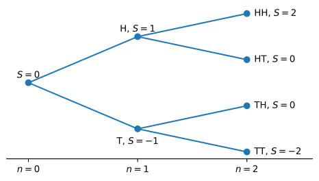
A filtration \mathcal{F}_{0} \subset \mathcal{F}_{1} \subset \mathcal{F}_{2} \subset \cdots describes information that accumulates and is never forgotten. With independent coin flips X_{n} = \pm 1 and \mathcal{F}_{n} generated by the first n flips, each flip splits every cell in two, as in Figure 1. The random walk S_{n} = X_{1} + \cdots + X_{n} is known at time n and the next flip is independent of \mathcal{F}_{n}, so \operatorname{E}(S_{n + 1} \mid \mathcal{F}_{n}) = S_{n} + \operatorname{E}(X_{n + 1}) = S_{n}. \tag{4} A process whose best forecast is its current value is a martingale.
Practice Problems
A portfolio holds two corporate bonds that default independently over the next year with probabilities 0.10 and 0.20. Let N be the number of defaults.
- Find the probability mass function of N.
- Compute \operatorname{E}(N) and \operatorname{V}(N).
- Given that at least one bond defaults, what is the probability that both default?
The economy expands next year with probability 0.7 and enters a recession with probability 0.3. A firm defaults with probability 2% in an expansion and 10% in a recession.
- Use the law of total probability to compute the probability that the firm defaults.
- Given that the firm defaults, what is the probability that the economy was in a recession?
Two random variables satisfy \operatorname{V}(X) = 4, \operatorname{V}(Y) = 9 and \operatorname{V}(X + Y) = 7.
- Compute \operatorname{Cov}(X, Y) and \rho_{X, Y}.
- Compute \operatorname{V}(X - Y) and \operatorname{V}(2 X - Y).
The table below describes two random variables on a sample space with four outcomes.
Outcome Probability X Y \omega_{1} 0.20 4 1 \omega_{2} 0.30 2 1 \omega_{3} 0.10 6 0 \omega_{4} 0.40 0 0 - Write down the partition generated by Y and list the events in \mathcal{F}_{Y}.
- Is Y^{2} known given \mathcal{F}_{Y}? Is X Y? Explain.
- Compute \operatorname{E}(X \mid \mathcal{F}_{Y}) on each cell and verify that \operatorname{E}(\operatorname{E}(X \mid \mathcal{F}_{Y})) = \operatorname{E}(X).
- Use the properties of conditional expectation to compute \operatorname{E}(X Y \mid \mathcal{F}_{Y}).
- Are X and Y independent? Explain.