Class 4

The Gambler’s Problem

A gambler bets one dollar on each flip of a fair coin. The flips X_{1}, X_{2}, \ldots are independent and equal to 1 or -1 with probability \frac{1}{2} each, so they have mean zero and variance one, and the gambler’s wealth is the random walk S_{n} = S_{0} + \sum_{i = 1}^{n} X_{i}. The gambler stops the first time the wealth reaches a target A or a floor -B, where A and B are positive integers: \tau = \min\{n > 0 : S_{n} = A \text{ or } S_{n} = -B\}. We want two numbers: the probability \operatorname{P}(S_{\tau} = A) of winning A dollars before losing B, and the expected duration \operatorname{E}(\tau) of the game.

The Game Ends

Both questions make sense only if the game ends. From any position strictly between -B and A, a streak of A + B wins reaches A. Split time into blocks of A + B flips. Each block is a winning streak with probability p = (1/2)^{A + B} > 0, independently of the other blocks, and the game can still be running after n blocks only if none of them was a streak. Therefore, \operatorname{P}(\tau > n (A + B)) \leq (1 - p)^{n} \xrightarrow[n \rightarrow \infty]{} 0, \tag{1} so \operatorname{P}(\tau = \infty) = 0. Writing \operatorname{E}(\tau) = \sum_{m = 0}^{\infty} \operatorname{P}(\tau > m), the same bound gives \operatorname{E}(\tau) \leq (A + B) / p < \infty, and in fact every moment of \tau is finite. The bound is crude, but it shows the questions have answers.

The Probability of Winning

The game has no clock, so the only state variable is the current wealth. Let f(K) = \operatorname{P}(S_{\tau} = A \mid S_{0} = K) for -B \leq K \leq A. Conditioning on the first flip, the gambler moves to K + 1 or K - 1 and the problem starts over from there: f(K) = \frac{1}{2} f(K - 1) + \frac{1}{2} f(K + 1), \qquad f(-B) = 0, \quad f(A) = 1. \tag{2} This is a second-order linear difference equation. Trying f(K) = z^{K} gives (z - 1)^{2} = 0, a repeated root, so the general solution is f(K) = \alpha + \beta K. The boundary conditions pin down the constants: f(K) = \frac{B + K}{A + B}, \qquad \operatorname{P}(S_{\tau} = A \mid S_{0} = 0) = \frac{B}{A + B}. \tag{3} A trade with a take-profit at +A and a stop-loss at -B on a fair random walk therefore has expected profit A \frac{B}{A + B} - B \frac{A}{A + B} = 0. The exit levels change the shape of the outcome, frequent small gains against rare large losses or the reverse, but not its mean.

Equations like (2) appear whenever a quantity depends only on the current state and the system moves to neighboring states with known probabilities. Pricing an option in a binomial tree works the same way.

The Expected Duration

Let g(K) = \operatorname{E}(\tau \mid S_{0} = K). One flip adds one period and moves the gambler to a neighboring state, so g(K) = 1 + \frac{1}{2} g(K - 1) + \frac{1}{2} g(K + 1), \qquad g(-B) = g(A) = 0. \tag{4} The homogeneous part is the same as before, and trying \gamma K^{2} gives the particular solution -K^{2}. Imposing the boundary conditions on \alpha + \beta K - K^{2}, g(K) = AB + (A - B) K - K^{2}, \qquad \operatorname{E}(\tau \mid S_{0} = 0) = AB. \tag{5} Doubling both barriers quadruples the expected duration. A random walk needs about n^{2} steps to travel a distance n, since its typical distance after m steps is of order \sqrt{m}: the scaling that turns a random walk into Brownian motion.

A Biased Coin

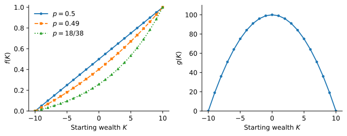
If each bet is won with probability p and lost with probability q = 1 - p, with p \neq q, the recursion becomes f(K) = p f(K + 1) + q f(K - 1). Trying z^{K} now gives p z^{2} - z + q = 0, with distinct roots z = 1 and z = q / p, so f(K) = \alpha + \beta (q / p)^{K} and f(K) = \frac{(q / p)^{K + B} - 1}{(q / p)^{A + B} - 1}. \tag{6} As p \to 1/2 this converges to the fair answer (K + B) / (A + B). Figure 1 shows how fast a small edge compounds: the gambler keeps betting until a barrier is reached, so the house edge accumulates over the whole game.

Figure 1: Left: probability f(K) of reaching A = 10 before -B = -10 from wealth K, for three probabilities p of winning each bet. Right: expected duration g(K) for the fair coin.

Practice Problems

1. A stock price moves up or down by $1 each period with probability 1/2. A trader buys one share and places a take-profit order $8 above the purchase price and a stop-loss order $4 below it.

   1. Compute the probability that the trade closes with the profit and the expected profit of the trade.
   2. Compute the expected number of periods until the trade closes.
   3. A few periods later the price is $2 above the purchase price and neither order has been executed. Compute the probability that the trade now closes with the profit and the expected number of remaining periods.
   4. Repeat the previous part if the price is instead $2 below the purchase price.

2. A thinly traded stock does not trade in half of the periods. Each period its price rises by $1 with probability 1/4, falls by $1 with probability 1/4, and stays unchanged with probability 1/2. A trader exits when the price is $6 above or $3 below the entry price. Let f(K) and g(K) be the probability of exiting with the profit and the expected number of periods to exit when the price is K dollars from the entry price.

   1. Condition on the first period to write the difference equations for f(K) and g(K), with their boundary conditions.
   2. Show that f(K) is the same as for the fair coin, and compute f(0).
   3. Show that g(K) = 2 \left(AB + (A - B) K - K^{2}\right) with A = 6 and B = 3, and compute g(0). Explain the factor of two.

3. A trading strategy gains $1 with probability p = 0.52 and loses $1 with probability q = 0.48 on each trade, independently. The trader has $50 of risk capital and stops after losing it or after making $50.

   1. Compute the probability of making $50 before losing $50 when the trader risks $1 per trade.
   2. Compute the same probability when the trader risks $5 per trade, so that each trade gains or loses $5 with the same probabilities.
   3. Compare your answers with the fair coin. Should a player with an edge make small or large bets?