Class 11

Discounted Prices Are Martingales

An asset with price p_{t} pays x_{t + 1} = p_{t + 1} + D_{t + 1} at time t + 1. Write \operatorname{E}_{t}(\cdot) for \operatorname{E}(\cdot \mid \mathcal{F}_{t}). If investors care only about expected payoffs, the price is p_{t} = \operatorname{E}_{t}(x_{t + 1}) / (1 + r), and dividing by (1 + r)^{t}, \frac{p_{t}}{(1 + r)^{t}} = \operatorname{E}_{t}\left(\frac{x_{t + 1}}{(1 + r)^{t + 1}}\right). Without dividends, the discounted price is a martingale: a fair price is a fair game.

Stochastic Discount Factors

Investors value a dollar more in a recession than in a boom, so an asset that pays off mostly in good times is worth less than its discounted expected payoff. Replacing the deterministic discount by a strictly positive random process \Lambda_{t}, the stochastic discount factor (SDF), gives \Lambda_{t} p_{t} = \operatorname{E}_{t}\left(\Lambda_{t + 1} x_{t + 1}\right). \tag{1} The same \Lambda prices every asset, and such a process exists in the absence of arbitrage. For a risk-free bond, \operatorname{E}_{t}(\Lambda_{t + 1}) / \Lambda_{t} = 1 / (1 + r): on average \Lambda discounts at the risk-free rate, and its randomness adjusts prices for risk.

Dividends keep \Lambda_{t} p_{t} from being a martingale, but reinvesting them fixes this. Holding X_{t} shares and buying more with each dividend, X_{t + 1} = X_{t} (1 + D_{t + 1} / p_{t + 1}), the position V_{t} = X_{t} p_{t} satisfies V_{t + 1} = X_{t} x_{t + 1}, so \Lambda_{t} V_{t} = \operatorname{E}_{t}\left(\Lambda_{t + 1} V_{t + 1}\right).

Prices, Dividends and the Money-Market Account

In continuous time, a risky asset follows \mathop{}\!\mathrm{d}S / S = \mu \mathop{}\!\mathrm{d}t+ \sigma \mathop{}\!\mathrm{d}B, where \mu and \sigma may be adapted processes, and \operatorname{E}_{t} extracts the drift: \operatorname{E}(\mathop{}\!\mathrm{d}S / S) = \mu \mathop{}\!\mathrm{d}t. The asset pays dividends at the rate D per unit of time, with dividend yield \delta = D / S. Reinvesting them, the number of shares grows at the dividend yield, \mathop{}\!\mathrm{d}X / X = (D / S) \mathop{}\!\mathrm{d}t, and since X has no diffusion term, the value V = X S of the position follows \frac{\mathop{}\!\mathrm{d}V}{V} = \frac{\mathop{}\!\mathrm{d}S}{S} + \frac{D}{S} \mathop{}\!\mathrm{d}t. A money-market account earns the risk-free rate r_{t}, which may itself be random: \frac{\mathop{}\!\mathrm{d}\beta_{t}}{\beta_{t}} = r_{t} \mathop{}\!\mathrm{d}t, \qquad \beta_{t} = \beta_{0} \exp\left(\int_{0}^{t} r_{s} \mathop{}\!\mathrm{d}s\right).

The Pricing Equation in Continuous Time

Letting the period shrink in \operatorname{E}_{t}(\Lambda_{t + \Delta t} V_{t + \Delta t} - \Lambda_{t} V_{t}) = 0 gives \operatorname{E}\mathop{}\!\mathrm{d}(\Lambda V) = 0, \qquad \text{equivalently} \qquad \operatorname{E}\mathop{}\!\mathrm{d}(\Lambda S) + \Lambda D \mathop{}\!\mathrm{d}t= 0. \tag{2} Since \Lambda and V are both Itô processes, the product rule is needed, and its cross term (\mathop{}\!\mathrm{d}\Lambda)(\mathop{}\!\mathrm{d}V) is the source of risk premia. The process \Lambda V has zero drift.

Applying (2) to the money-market account, which pays no dividends and has no diffusion term, \mathop{}\!\mathrm{d}(\Lambda \beta) = \Lambda \mathop{}\!\mathrm{d}\beta + \beta \mathop{}\!\mathrm{d}\Lambda and \operatorname{E}\left(\frac{\mathop{}\!\mathrm{d}\Lambda}{\Lambda}\right) = -r \mathop{}\!\mathrm{d}t. \tag{3} The drift of the SDF is minus the risk-free rate. Applying the product rule to \Lambda S and taking drifts then gives the central result.

WarningFundamental Pricing Equation

If \mathop{}\!\mathrm{d}S / S = \mu \mathop{}\!\mathrm{d}t+ \sigma \mathop{}\!\mathrm{d}B, the asset has dividend yield \delta = D / S, and there are no arbitrage opportunities, (\mu + \delta - r) \mathop{}\!\mathrm{d}t= -\left(\frac{\mathop{}\!\mathrm{d}\Lambda}{\Lambda}\right) \left(\frac{\mathop{}\!\mathrm{d}S}{S}\right). \tag{4} The risk premium equals minus the instantaneous covariance of the SDF with the asset’s return.

An asset that pays off poorly when the SDF is high, in bad times, covaries negatively with the SDF and must offer an expected return above r. If the SDF has no diffusion term, every asset earns the risk-free rate.

Specifying the SDF

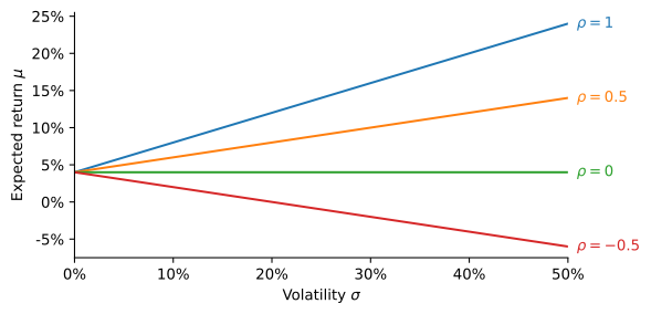
Write \mathop{}\!\mathrm{d}\Lambda / \Lambda = -r \mathop{}\!\mathrm{d}t- \lambda \mathop{}\!\mathrm{d}B_{1}, and let the stock be driven by B_{2} with (\mathop{}\!\mathrm{d}B_{1})(\mathop{}\!\mathrm{d}B_{2}) = \rho \mathop{}\!\mathrm{d}t. For a stock without dividends, (4) gives \mu - r = \lambda \rho \sigma. \tag{5} Only the part of volatility correlated with the SDF earns a premium, as Figure 1 shows. When the stock and the SDF share one Brownian motion, \rho = 1 and \lambda = (\mu - r) / \sigma: the volatility of the SDF is the instantaneous Sharpe ratio, common to every asset driven by that Brownian motion. A stock with \rho = 0 earns r however volatile it is, and one with \rho < 0 earns less than r.

Figure 1: Expected returns from \mu = r + \lambda \rho \sigma with r = 4\% and SDF volatility \lambda = 0.4, for four correlations between the stock and the SDF shock.

In a consumption-based model, the SDF is discounted marginal utility. With power utility, \Lambda_{t} = e^{-\phi t} C_{t}^{-\gamma}, and if consumption follows \mathop{}\!\mathrm{d}C / C = \mu_{C} \mathop{}\!\mathrm{d}t+ \sigma_{C} \mathop{}\!\mathrm{d}B_{C}, Itô’s lemma for powers of a GBM gives r = \phi + \gamma \mu_{C} - \tfrac{1}{2} \gamma (\gamma + 1) \sigma_{C}^{2}, \qquad \mu + \delta - r = \gamma \rho \sigma_{C} \sigma, \tag{6} where \rho is the correlation of the stock’s return with consumption growth. Since consumption is smooth, matching the historical equity premium requires an implausibly high \gamma, the equity premium puzzle.

Practice Problems

1. Next year the economy is in a boom or a recession with equal probability. The SDF is \Lambda_{0} = 1 today, and \Lambda_{1} = 0.88 in the boom and \Lambda_{1} = 1.04 in the recession.

   1. Compute the price of a bond that pays $1 in both states and the risk-free rate.
   2. A stock pays $120 in the boom and $80 in the recession. Compute its price and its expected return, and compare the price with the expected payoff discounted at the risk-free rate.
   3. An insurance contract pays $20 in the recession and nothing in the boom. Compute its price and its expected return. Why is the expected return below the risk-free rate?

2. A stock pays a constant dividend yield \delta = 2\% and follows \mathop{}\!\mathrm{d}S / S = \mu \mathop{}\!\mathrm{d}t+ \sigma \mathop{}\!\mathrm{d}B with \sigma = 20\%. The SDF follows \mathop{}\!\mathrm{d}\Lambda / \Lambda = -r \mathop{}\!\mathrm{d}t- \lambda \mathop{}\!\mathrm{d}B with r = 3\% and \lambda = 0.35.

   1. An investor holds 100 shares and reinvests all dividends. How many shares does the investor hold after ten years?
   2. Use (4) to find the expected return \mu of the stock and the drift of the reinvested position V.
   3. Use the product rule to write the process followed by \Lambda V, and verify that it has zero drift.

3. The SDF follows \mathop{}\!\mathrm{d}\Lambda / \Lambda = -r \mathop{}\!\mathrm{d}t- \lambda \mathop{}\!\mathrm{d}B_{1} with r = 4\% and \lambda = 0.5. Three stocks without dividends have volatilities and correlations with B_{1} given below.

   Stock	\sigma	\rho
   A	20%	0.8
   B	40%	0.2
   C	15%	-0.2

   1. Compute the risk premium, the expected return and the Sharpe ratio of each stock.
   2. Stock B is twice as volatile as stock A. Explain why its expected return is lower.
   3. A fourth stock has a volatility of 30% and an expected return of 4%. What is its correlation with B_{1}?