Class 7

Modified

October 22, 2026

From Random Walks to Brownian Motion

Prices move all the time by small amounts, which the Poisson process cannot capture. Start from fair coin flips X_{i} = \pm 1, divide time into slots of length \Delta t, and move up or down by \sqrt{\Delta t} at the end of each slot. At time t = m \Delta t the scaled random walk is B_{t}^{(n)} = \sqrt{\Delta t} \, (X_{1} + \cdots + X_{m}), with n = 1 / \Delta t steps per unit of time, and \operatorname{E}(B_{t}^{(n)}) = 0, \qquad \operatorname{V}(B_{t}^{(n)}) = t, \qquad [B^{(n)}, B^{(n)}]_{t} = \sum_{j = 1}^{m} (\sqrt{\Delta t} \, X_{j})^{2} = t. The step \sqrt{\Delta t} is the only one that keeps the variance at t: smaller steps make the walk collapse and larger ones make it explode. The characteristic function \cos(u \sqrt{\Delta t})^{t / \Delta t} converges to e^{-\frac{1}{2} u^{2} t}, so B_{t}^{(n)} converges to \mathcal{N}(0, t), and increments over disjoint intervals stay independent in the limit.

Brownian Motion

A Brownian motion \{B_{t}\} satisfies B_{0} = 0, has independent increments, has B_{t} - B_{s} \sim \mathcal{N}(0, t - s) for s < t, and has continuous paths with probability one. The first two properties are those of the Poisson process, the normal increment replaces the Poisson one, and continuity rules out jumps. Writing B_{t} = B_{s} + (B_{t} - B_{s}) for s \leq t gives \operatorname{E}(B_{t}) = 0, \qquad \operatorname{V}(B_{t}) = t, \qquad \operatorname{Cov}(B_{s}, B_{t}) = \min(s, t). \tag{1} The correlation between B_{s} and B_{t} is \sqrt{s / t}, which depends on the ratio of the dates rather than on the gap between them. Over a short interval the increment \mathop{}\!\mathrm{d}B_{t} has standard deviation \sqrt{\mathop{}\!\mathrm{d}t}, far larger than \mathop{}\!\mathrm{d}t, so a Brownian path is never flat.

Martingales of Brownian Motion

With \mathcal{F}_{t} generated by the path up to t, each future increment \Delta B = B_{t} - B_{s} is independent of \mathcal{F}_{s}, with \operatorname{E}(\Delta B) = 0, \operatorname{E}(\Delta B^{2}) = t - s and \operatorname{E}(e^{\theta \Delta B}) = e^{\frac{1}{2} \theta^{2} (t - s)}. These three facts show that B_{t}, \qquad B_{t}^{2} - t, \qquad Z_{t} = \exp\left(\theta B_{t} - \tfrac{1}{2} \theta^{2} t\right) \tag{2} are martingales, with proofs identical line by line to those for the Poisson process. The exponential martingale has the form e^{\theta B_{t} - t K(\theta)}, where K(\theta) = \frac{1}{2} \theta^{2} is the CGF of B_{1}.

Hitting a Barrier

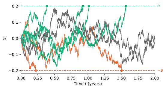
Default, knock-out options and drawdown limits all ask whether a process reaches a level. Model a log value as a Brownian motion with drift X_{t} = \mu t + \sigma B_{t}, and let \tau be the first time it reaches -a < 0 or b > 0. Applying (2) with \theta \sigma in place of \theta and choosing \theta = -\gamma, where \gamma = 2 \mu / \sigma^{2}, removes the time term and makes e^{-\gamma X_{t}} a martingale. Stopping it at \tau, where X_{\tau} equals -a or b exactly because paths are continuous, gives \operatorname{P}(X_{\tau} = -a) = \frac{1 - e^{-\gamma b}}{e^{\gamma a} - e^{-\gamma b}}. \tag{3} If \mu > 0, letting b \to \infty gives the probability e^{-\gamma a} of ever reaching -a, and as \mu \to 0 the formula tends to b / (a + b), the fair gambler’s ruin probability. For the insurer the surplus jumps past zero, so Lundberg’s argument gives only a bound. Here continuity makes the answer exact. Figure 1 shows paths stopped at the two barriers.

Eight rough paths start at zero and wander between two dashed horizontal lines, an upper barrier b at 0.2 and a lower barrier minus a at minus 0.2, over two years. Four green paths end with a dot on the upper barrier, two orange paths end with a dot on the lower barrier, and two gray paths have not reached either barrier by year 2. — Figure 1: Eight simulated paths of X_{t} = \mu t + \sigma B_{t} with \mu = 0.05 and \sigma = 0.20, each stopped when it reaches -a = -0.2 or b = 0.2. By (3) a path reaches -a first with probability 0.38.

Quadratic Variation

For a partition 0 = t_{0} < \cdots < t_{n} = T with mesh \lVert{\Pi}\rVert, the total variation adds up |f(t_{j + 1}) - f(t_{j})| and the quadratic variation adds up (f(t_{j + 1}) - f(t_{j}))^{2}. A smooth function moves by an amount proportional to t_{j + 1} - t_{j}, so it has finite total variation and zero quadratic variation. Brownian motion moves by about \sqrt{t_{j + 1} - t_{j}}, and the sum of squared increments Q_{\Pi} satisfies \operatorname{E}(Q_{\Pi}) = T, \qquad \operatorname{V}(Q_{\Pi}) \leq 2 \lVert{\Pi}\rVert T, \qquad [B, B]_{T} = T. \tag{4} The limit is essentially the same on every path, unlike the random [N, N]_{t} = N_{t} of the Poisson process. Together with sums of \mathop{}\!\mathrm{d}B \mathop{}\!\mathrm{d}t and (\mathop{}\!\mathrm{d}t)^{2} that vanish, this gives the multiplication table (\mathop{}\!\mathrm{d}B)^{2} = \mathop{}\!\mathrm{d}t, \qquad (\mathop{}\!\mathrm{d}B)(\mathop{}\!\mathrm{d}t) = 0, \qquad (\mathop{}\!\mathrm{d}t)^{2} = 0.

Since Q_{\Pi} \leq M_{\Pi} \sum_{j} |B_{t_{j + 1}} - B_{t_{j}}|, where M_{\Pi} is the largest move and tends to zero, the total variation of Brownian motion is infinite and its paths are smooth on no interval. This is why sums \sum f(t_{j}) (B_{t_{j + 1}} - B_{t_{j}}) that approximate an integral against B depend on where in each subinterval the integrand is evaluated, and why stochastic calculus needs its own rules.

Practice Problems

A model of intraday trading moves the log price of a stock up or down by h every period, with probability 1/2 each, and there are n = 10{,}000 periods per year.
1. Find the step size h that gives the log price a variance of \sigma^{2} = 0.04 over one year.
2. Compute the quadratic variation of the log price over one year. Does it depend on the path?
3. Use the normal limit to approximate the probability that the log price rises by more than 0.3 over the year.
4. Compute the total distance the log price travels over the year, the sum of the absolute values of all its moves, and compare it with the typical size of the change in the log price over the year. What happens to this distance as n \to \infty with \sigma^{2} fixed?
Let \{B_{t}\} be a Brownian motion, and suppose that B_{1} = 0.5 has been observed.
1. Use (2) to compute \operatorname{E}(B_{3} \mid \mathcal{F}_{1}), \operatorname{E}(B_{3}^{2} \mid \mathcal{F}_{1}), and \operatorname{E}(e^{B_{3}} \mid \mathcal{F}_{1}).
2. Find the constant c such that e^{2 B_{t} - c t} is a martingale, and use it to compute \operatorname{E}(e^{2 B_{t}}).
3. Decide whether each process is a martingale, and justify your answer: (i) t B_{t}, (ii) B_{t}^{2} - t + 5, (iii) e^{B_{t} - t}.
A trader’s cumulative log return on a position follows X_{t} = \mu t + \sigma B_{t}, with \mu = 0.10 and \sigma = 0.20 per year. The trader closes the position with a stop-loss when the log return reaches -0.10 and takes profits when it reaches 0.20.
1. Compute \gamma, and the probability that the stop-loss is triggered before the profit target.
2. Repeat the calculation for a trader with no skill, \mu = 0, and comment on how much the drift matters.
3. Suppose the trader drops the profit target. Compute the probability that the stop-loss is ever triggered.
4. Without a profit target, how far below zero must the stop-loss be set for the probability of ever triggering it to be 10%?