Class 9
Itô’s Formula: A Reminder
For an Itô process \mathop{}\!\mathrm{d}X_{t} = a_{t} \mathop{}\!\mathrm{d}t+ b_{t} \mathop{}\!\mathrm{d}B_{t} and a smooth function f(x, t), Itô’s formula reads \mathop{}\!\mathrm{d}f(X_{t}, t) = \frac{\partial f}{\partial t} \mathop{}\!\mathrm{d}t+ \frac{\partial f}{\partial x} \mathop{}\!\mathrm{d}X_{t} + \frac{1}{2} \frac{\partial^{2} f}{\partial x^{2}} (\mathop{}\!\mathrm{d}X_{t})^{2}, \qquad (\mathop{}\!\mathrm{d}X_{t})^{2} = b_{t}^{2} \mathop{}\!\mathrm{d}t. \tag{1} Today we extend it to several processes driven by different, possibly correlated, sources of risk, and then see how changing the probability measure changes the drift of a Brownian motion.
Correlated Brownian Motions
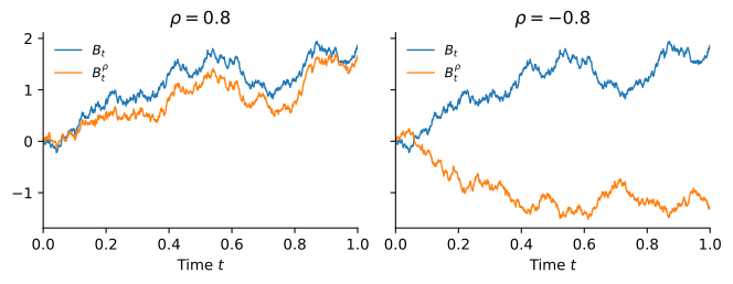
Asset pricing models usually involve several sources of risk, such as a stock price and an interest rate. If B_{t} and W_{t} are independent Brownian motions, the sum \sum_{j} \Delta B_{j} \Delta W_{j} has mean zero and variance \sum_{j} \Delta t_{j}^{2} \leq \lVert{\Pi}\rVert t, so it vanishes in the limit and (\mathop{}\!\mathrm{d}B_{t})(\mathop{}\!\mathrm{d}W_{t}) = 0. For -1 \leq \rho \leq 1, is again a Brownian motion: its increments are independent and normal with variance (\rho^{2} + 1 - \rho^{2})(t - s) = t - s. Its increments have correlation \rho with those of B_{t}, and (\mathop{}\!\mathrm{d}B_{t})(\mathop{}\!\mathrm{d}B_{t}^{\rho}) = \rho (\mathop{}\!\mathrm{d}B_{t})^{2} + \sqrt{1 - \rho^{2}} \, (\mathop{}\!\mathrm{d}B_{t})(\mathop{}\!\mathrm{d}W_{t}) = \rho \mathop{}\!\mathrm{d}t. Figure 1 builds B^{\rho} from the same two paths for \rho = 0.8 and \rho = -0.8.
Writing B_{1} and B_{2} for two Brownian motions whose increments have correlation \rho, the multiplication table is:
| Product | \mathop{}\!\mathrm{d}t | \mathop{}\!\mathrm{d}B_{1} | \mathop{}\!\mathrm{d}B_{2} |
|---|---|---|---|
| \mathop{}\!\mathrm{d}t | 0 | 0 | 0 |
| \mathop{}\!\mathrm{d}B_{1} | 0 | \mathop{}\!\mathrm{d}t | \rho \mathop{}\!\mathrm{d}t |
| \mathop{}\!\mathrm{d}B_{2} | 0 | \rho \mathop{}\!\mathrm{d}t | \mathop{}\!\mathrm{d}t |
For \mathop{}\!\mathrm{d}X_{t} = a_{t} \mathop{}\!\mathrm{d}t+ b_{t} \mathop{}\!\mathrm{d}B_{1} and \mathop{}\!\mathrm{d}Y_{t} = c_{t} \mathop{}\!\mathrm{d}t+ d_{t} \mathop{}\!\mathrm{d}B_{2}, the table gives the instantaneous covariance (\mathop{}\!\mathrm{d}X_{t})(\mathop{}\!\mathrm{d}Y_{t}) = \rho \, b_{t} d_{t} \mathop{}\!\mathrm{d}t, \tag{3} so the instantaneous correlation of \mathop{}\!\mathrm{d}X_{t} and \mathop{}\!\mathrm{d}Y_{t} is \rho when b_{t} and d_{t} are positive.
Itô’s Formula for Two Processes
For a smooth function f(x, y, t), the second-order expansion picks up a cross term: \mathop{}\!\mathrm{d}f = \frac{\partial f}{\partial t} \mathop{}\!\mathrm{d}t+ \frac{\partial f}{\partial x} \mathop{}\!\mathrm{d}X + \frac{\partial f}{\partial y} \mathop{}\!\mathrm{d}Y + \frac{1}{2} \frac{\partial^{2} f}{\partial x^{2}} (\mathop{}\!\mathrm{d}X)^{2} + \frac{\partial^{2} f}{\partial x \partial y} (\mathop{}\!\mathrm{d}X)(\mathop{}\!\mathrm{d}Y) + \frac{1}{2} \frac{\partial^{2} f}{\partial y^{2}} (\mathop{}\!\mathrm{d}Y)^{2}. \tag{4} With f(x, y) = x y it gives the product rule, and for positive processes its version in percentage changes: \mathop{}\!\mathrm{d}(X_{t} Y_{t}) = X_{t} \mathop{}\!\mathrm{d}Y_{t} + Y_{t} \mathop{}\!\mathrm{d}X_{t} + (\mathop{}\!\mathrm{d}X_{t})(\mathop{}\!\mathrm{d}Y_{t}), \qquad \frac{\mathop{}\!\mathrm{d}(X_{t} Y_{t})}{X_{t} Y_{t}} = \frac{\mathop{}\!\mathrm{d}X_{t}}{X_{t}} + \frac{\mathop{}\!\mathrm{d}Y_{t}}{Y_{t}} + \left(\frac{\mathop{}\!\mathrm{d}X_{t}}{X_{t}}\right)\left(\frac{\mathop{}\!\mathrm{d}Y_{t}}{Y_{t}}\right). \tag{5} The correction vanishes when either process has no diffusion term. For a stock with \mathop{}\!\mathrm{d}S_{t} / S_{t} = \mu \mathop{}\!\mathrm{d}t+ \sigma \mathop{}\!\mathrm{d}B_{t} and a money-market account \beta_{t} = e^{r t}, the discount factor 1 / \beta_{t} has no diffusion, so \frac{\mathop{}\!\mathrm{d}(S_{t} / \beta_{t})}{S_{t} / \beta_{t}} = (\mu - r) \mathop{}\!\mathrm{d}t+ \sigma \mathop{}\!\mathrm{d}B_{t}. \tag{6} The discounted stock has drift equal to the expected excess return and the same volatility as the stock.
Girsanov’s Theorem
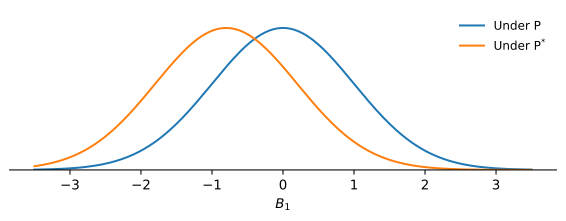
To make discounted prices martingales we want to remove the drift in (6) without touching the paths. For a constant \theta and horizon T, the exponential martingale Z_{t} = \exp\left(-\theta B_{t} - \frac{1}{2} \theta^{2} t\right) is positive with \operatorname{E}(Z_{T}) = 1, so it defines a new probability measure \operatorname{P}^{*}(A) = \operatorname{E}\left(Z_{T} \mathbf{1}_{\{A\}}\right), \qquad \operatorname{E}^{*}(Y) = \operatorname{E}(Z_{T} Y). \tag{7} Girsanov’s theorem states that under \operatorname{P}^{*}, B_{t}^{*} = B_{t} + \theta t is a Brownian motion for 0 \leq t \leq T. The same holds for an adapted \theta_{t} with B_{t}^{*} = B_{t} + \int_{0}^{t} \theta_{s} \mathop{}\!\mathrm{d}s, as long as the corresponding Z_{t} is a martingale, for instance when \theta_{t} is bounded. When \theta > 0, paths that end high get less weight, which shifts the distribution of B_{t} down, as in Figure 2.
In differential form, \mathop{}\!\mathrm{d}B_{t} = \mathop{}\!\mathrm{d}B_{t}^{*} - \theta \mathop{}\!\mathrm{d}t, so an Itô process becomes \mathop{}\!\mathrm{d}X_{t} = (a_{t} - \theta b_{t}) \mathop{}\!\mathrm{d}t+ b_{t} \mathop{}\!\mathrm{d}B_{t}^{*} \tag{8} under \operatorname{P}^{*}. The drift shifts by -\theta b_{t} and the volatility is unchanged: quadratic variation is computed path by path, and \operatorname{P}^{*} reweights paths without changing them. Since Z_{T} > 0, the two measures agree on which events are impossible. Choosing \theta = (\mu - r) / \sigma, the instantaneous Sharpe ratio, removes the drift in (6), and the stock follows \mathop{}\!\mathrm{d}S_{t} / S_{t} = r \mathop{}\!\mathrm{d}t+ \sigma \mathop{}\!\mathrm{d}B_{t}^{*} under \operatorname{P}^{*}. This is the construction behind the risk-neutral measure.
Practice Problems
A US investor holds a European stock. Its price in euros follows \mathop{}\!\mathrm{d}S_{t} / S_{t} = \mu_{S} \mathop{}\!\mathrm{d}t+ \sigma_{S} \mathop{}\!\mathrm{d}B_{1}, and the exchange rate in dollars per euro follows \mathop{}\!\mathrm{d}X_{t} / X_{t} = \mu_{X} \mathop{}\!\mathrm{d}t+ \sigma_{X} \mathop{}\!\mathrm{d}B_{2}, where the increments of B_{1} and B_{2} have correlation \rho. The dollar price of the stock is D_{t} = X_{t} S_{t}.
- Use the product rule to find \mathop{}\!\mathrm{d}D_{t} / D_{t}.
- With \mu_{S} = 8\%, \sigma_{S} = 25\%, \mu_{X} = 1\%, \sigma_{X} = 10\% and \rho = -0.3, compute the drift and the volatility of the dollar return.
Let B_{t} and W_{t} be independent Brownian motions, and define X_{t} = 0.6 B_{t} + 0.8 W_{t} and Y_{t} = 0.6 B_{t} - 0.8 W_{t}.
- Compute (\mathop{}\!\mathrm{d}B_{t})(\mathop{}\!\mathrm{d}X_{t}) and (\mathop{}\!\mathrm{d}X_{t})(\mathop{}\!\mathrm{d}Y_{t}).
- Use the product rule to find the drift of B_{t} X_{t}, and compute \operatorname{E}(B_{t} X_{t}).
- Express W_{t} in terms of B_{t} and X_{t}.
A portfolio manager’s position, in millions of dollars, follows \mathop{}\!\mathrm{d}V_{t} = \mu_{V} \mathop{}\!\mathrm{d}t+ 3 \mathop{}\!\mathrm{d}B_{1}, and the price of a stock index futures contract follows \mathop{}\!\mathrm{d}F_{t} = \mu_{F} \mathop{}\!\mathrm{d}t+ 2 \mathop{}\!\mathrm{d}B_{2}, where the increments of B_{1} and B_{2} have correlation \rho = 0.8. The manager sells h units of the futures, so the hedged position is H_{t} = V_{t} - h F_{t}.
- Compute (\mathop{}\!\mathrm{d}H_{t})^{2} as a function of h.
- Find the hedge ratio h that minimizes the instantaneous variance of the hedged position.
- Compute the instantaneous standard deviation of the hedged position at that h, and the fraction of the original variance the hedge removes.
The value of a firm’s assets follows \mathop{}\!\mathrm{d}V_{t} / V_{t} = \mu \mathop{}\!\mathrm{d}t+ \sigma \mathop{}\!\mathrm{d}B_{t} with \mu = 10\% and \sigma = 20\%, and the risk-free rate is r = 4\%.
- Find the \theta that makes V_{t} / \beta_{t} have zero drift under \operatorname{P}^{*}, and write the process followed by V_{t} under \operatorname{P}^{*}.
- Find the distribution of \ln (V_{1} / V_{0}) under \operatorname{P} and under \operatorname{P}^{*}.
- Compute the probability that the assets lose more than 25% of their value by time 1 under \operatorname{P} and under \operatorname{P}^{*}. Why is one larger?