Class 3
Probability Generating Functions
Most random variables in this course are sums: a random walk is a sum of flips, defaults in a loan book are a sum of indicators, and an annual log return is a sum of daily ones. A generating function encodes a whole distribution in one function and turns sums of independent variables into products. For X taking values in \mathbb{N} = \{0, 1, 2, \ldots\}, the probability generating function (PGF) is G_{X}(z) = \operatorname{E}(z^{X}) = \sum_{k = 0}^{\infty} p_{X}(k) z^{k}, \qquad G_{X}(1) = 1. \tag{1} The coefficient of z^{k} is \operatorname{P}(X = k) = G_{X}^{(k)}(0) / k!, so the PGF determines the distribution: if we recognize a PGF, we know the distribution. Setting z = 1 in the derivatives gives the moments, \operatorname{E}(X) = G_{X}'(1), \qquad \operatorname{V}(X) = G_{X}''(1) + G_{X}'(1) - G_{X}'(1)^{2}. \tag{2} Three PGFs cover most of what we need: Bernoulli 1 - p + p z, geometric (flips until the first head) p z / (1 - q z) with q = 1 - p, and Poisson e^{\lambda (z - 1)}.
Sums, Random Sums and the Poisson Limit
If X and Y are independent, then G_{X + Y}(z) = G_{X}(z) \, G_{Y}(z). Multiplying the power series performs every convolution sum \sum_{j} p_{X}(j) p_{Y}(k - j) at once. A sum of n Bernoulli defaults has PGF (1 - p + p z)^{n}, the binomial distribution, and independent Poisson counts add up to a Poisson count with the summed parameter.
When the number of terms N is itself random and independent of the iid terms X_{1}, X_{2}, \ldots, the random sum S = X_{1} + \cdots + X_{N} has G_{S}(z) = G_{N}(G_{X}(z)), \qquad \operatorname{E}(S) = \operatorname{E}(N) \operatorname{E}(X). \tag{3} Thinning a \text{Poisson}(\lambda) count, keeping each event with probability p, gives \text{Poisson}(\lambda p).
With n loans that each default with probability p = \lambda / n, the binomial PGF is (1 + \lambda (z - 1) / n)^{n} \to e^{\lambda (z - 1)}. By the continuity theorem for PGFs the probabilities converge too: many independent rare events produce an approximately Poisson count with parameter equal to the expected number of events, the law of rare events.
Moment Generating Functions
Substituting z = e^{\theta} handles variables with negative or continuous values. The moment generating function (MGF) is M_{X}(\theta) = \operatorname{E}(e^{\theta X}), wherever it is finite. When it is finite near zero:
- \operatorname{E}(X^{k}) = M_{X}^{(k)}(0).
- M_{a + b X}(\theta) = e^{a \theta} M_{X}(b \theta).
- If X and Y are independent, M_{X + Y}(\theta) = M_{X}(\theta) M_{Y}(\theta).
- The MGF determines the distribution.
The key cases are T \sim \text{Exp}(\lambda) : \ \frac{\lambda}{\lambda - \theta}, \qquad X \sim \text{Gamma}(\alpha, \lambda) : \ \left(\frac{\lambda}{\lambda - \theta}\right)^{\alpha}, \qquad X \sim \mathcal{N}(\mu, \sigma^{2}) : \ e^{\mu \theta + \frac{1}{2} \sigma^{2} \theta^{2}}, \tag{4} the first two for \theta < \lambda. Products of these give three facts at once: a sum of n independent \text{Exp}(\lambda) waiting times is \text{Gamma}(n, \lambda), Z_{1}^{2} + \cdots + Z_{k}^{2} is chi-squared \text{Gamma}(k/2, 1/2), and independent normals sum to a normal, so independent normal daily log returns give a normal annual log return. Lognormal moments are values of the normal MGF, \operatorname{E}(e^{\alpha X}) = M_{X}(\alpha). The lognormal variable e^{X} itself has no MGF, and neither does a Student t.
Cumulant Generating Functions
The cumulant generating function K_{X}(\theta) = \ln M_{X}(\theta) turns independent sums into sums, K_{X + Y} = K_{X} + K_{Y}, and K_{X}'(0) = \operatorname{E}(X), \qquad K_{X}''(0) = \operatorname{V}(X). \tag{5} The normal has K(\theta) = \mu \theta + \frac{1}{2} \sigma^{2} \theta^{2}, so its cumulants beyond the variance are zero, and the Poisson has K(\theta) = \lambda (e^{\theta} - 1). For iid steps with cumulant generating function K, the process e^{\theta S_{n} - n K(\theta)} is an exponential martingale, the tool we will use for stopping times and changes of measure.
Characteristic Functions and the CLT
The characteristic function \phi_{X}(u) = \operatorname{E}(e^{i u X}) = \operatorname{E}(\cos(u X)) + i \, \operatorname{E}(\sin(u X)) exists for every random variable, since |\phi_{X}(u)| \leq 1. It shares the MGF properties: \phi_{a + b X}(u) = e^{i a u} \phi_{X}(b u), independent sums multiply, it determines the distribution, and \phi_{X}^{(k)}(0) = i^{k} \operatorname{E}(X^{k}). For integer-valued X, \operatorname{P}(X = k) = \frac{1}{2 \pi} \int_{-\pi}^{\pi} e^{-i u k} \phi_{X}(u) \, du. The normal has \phi(u) = e^{i \mu u - \frac{1}{2} \sigma^{2} u^{2}} and a fair \pm 1 coin has \phi(u) = \cos(u).
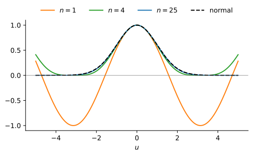
By Lévy’s continuity theorem, X_{n} converges in distribution to X exactly when \phi_{X_{n}}(u) \to \phi_{X}(u) for every u. For iid X_{i} with mean zero and variance \sigma^{2}, a Taylor expansion gives \phi_{S_{n} / \sqrt{n}}(u) = \left(1 - \frac{\sigma^{2} u^{2}}{2 n} + o\left(\frac{1}{n}\right)\right)^{n} \longrightarrow e^{-\frac{1}{2} \sigma^{2} u^{2}}, \tag{6} the central limit theorem. Figure 1 shows it for the coin: \cos(u / \sqrt{n})^{n} approaches e^{-u^{2}/2}. The Poisson limit has the same structure, a transform raised to the n-th power with (1 + x / n)^{n} \to e^{x}, but rare events give a count while small shocks give a normal.
Practice Problems
The number of defaults N next year in a loan book has the PGF G_{N}(z) = e^{3 (z - 1)} (0.7 + 0.3 z)^{2}.
- Interpret N as a sum of independent counts: what distributions and parameters are involved?
- Compute \operatorname{E}(N) and \operatorname{V}(N).
- Compute \operatorname{P}(N = 0) and \operatorname{P}(N = 1).
A hedge fund closes at the end of each year with probability 0.2, so the number of years N it operates, including the year it closes, is geometric with p = 0.2. In each year of operation the fund beats its benchmark with probability 0.5, independently of other years and of N. Let S be the number of years in which the fund beats its benchmark.
- Show that G_{S}(z) = \dfrac{1 + z}{6 - 4 z}.
- Compute \operatorname{E}(S) and \operatorname{V}(S).
- Compute \operatorname{P}(S = 0), and show that \operatorname{P}(S = k) = \frac{5}{18} \left(\frac{2}{3}\right)^{k - 1} for k \geq 1.
A catastrophe bond defaults at the third hurricane landfall in a region. The times between landfalls are independent and exponential with rate \lambda = 0.5 per year, and W is the time to the third landfall.
- Find the MGF of W and identify its distribution.
- Use the cumulant generating function of W to compute \operatorname{E}(W) and \operatorname{SD}(W).
- Use the MGF to find the distribution of the same time measured in months, 12 W.
A stock’s annual log return is R = 0.08 + 0.20 Z - 0.10 N, where Z \sim \mathcal{N}(0, 1) and the number of crashes N \sim \text{Poisson}(0.5) are independent. Each crash lowers the log price by 0.10.
- Find the cumulant generating function K_{R}(\theta).
- Use it to compute \operatorname{E}(R) and \operatorname{V}(R).
- Compute the expected gross return \operatorname{E}(e^{R}).
- Compute the third cumulant K_{R}'''(0). What does its sign say about the distribution of R, compared with a normal log return?