Class 10

Geometric Brownian Motion

A Brownian motion can turn negative, and its changes do not depend on its level. Stock prices are positive, and a stock at $200 moves about twice as many dollars in a day as the same stock at $100. What is roughly stable is the distribution of returns, so the standard model lets returns follow a Brownian motion with drift: \frac{\mathop{}\!\mathrm{d}S_{t}}{S_{t}} = \mu \mathop{}\!\mathrm{d}t+ \sigma \mathop{}\!\mathrm{d}B_{t}, \qquad \text{or} \qquad \mathop{}\!\mathrm{d}S_{t} = \mu S_{t} \mathop{}\!\mathrm{d}t+ \sigma S_{t} \mathop{}\!\mathrm{d}B_{t}. \tag{1} The process \{S_{t}\} is a geometric Brownian motion (GBM). The constant \mu is the expected return per unit of time and \sigma is the volatility of returns, both usually quoted per year. Over a short interval \Delta t, the return \Delta S_{t} / S_{t} is approximately normal with mean \mu \Delta t and variance \sigma^{2} \Delta t.

Solving for the Stock Price

Itô’s lemma applied to X_{t} = \ln S_{t}, with f'(S) = 1 / S, f''(S) = -1 / S^{2} and (\mathop{}\!\mathrm{d}S_{t})^{2} = \sigma^{2} S_{t}^{2} \mathop{}\!\mathrm{d}t, gives \mathop{}\!\mathrm{d}\ln S_{t} = \frac{\mathop{}\!\mathrm{d}S_{t}}{S_{t}} - \frac{1}{2} \frac{(\mathop{}\!\mathrm{d}S_{t})^{2}}{S_{t}^{2}} = \left(\mu - \tfrac{1}{2} \sigma^{2}\right) \mathop{}\!\mathrm{d}t+ \sigma \mathop{}\!\mathrm{d}B_{t}. The log price is a Brownian motion with drift, and integrating from 0 to T, S_{T} = S_{0} \exp\left(\left(\mu - \tfrac{1}{2} \sigma^{2}\right) T + \sigma B_{T}\right). \tag{2} The term -\frac{1}{2} \sigma^{2} is the Itô correction: ordinary calculus would wrongly give the log price a drift of \mu. Equivalently, S_{t} = S_{0} e^{\mu t} Z_{t}, where Z_{t} = \exp\left(\sigma B_{t} - \frac{1}{2} \sigma^{2} t\right) is the exponential martingale, with \mathop{}\!\mathrm{d}Z_{t} = \sigma Z_{t} \mathop{}\!\mathrm{d}B_{t}.

The Distribution of the Stock Price

Since B_{T} \sim \mathcal{N}(0, T), (2) implies \ln S_{T} \sim \mathcal{N}\left(\ln S_{0} + \left(\mu - \tfrac{1}{2} \sigma^{2}\right) T, \, \sigma^{2} T\right), \tag{3} so S_{T} is lognormal. The continuously compounded return \ln(S_{T} / S_{0}) is normal with mean \left(\mu - \frac{1}{2} \sigma^{2}\right) T and standard deviation \sigma \sqrt{T}. To compute a probability about the price, translate it into a statement about this normal return and standardize. For instance, \operatorname{P}(S_{T} > K) = \operatorname{P}\left(Z > \frac{\ln(K / S_{0}) - \left(\mu - \frac{1}{2} \sigma^{2}\right) T}{\sigma \sqrt{T}}\right), where Z is standard normal. Probability intervals for \ln S_{T} become intervals for S_{T} by exponentiating the endpoints, and they are not symmetric around the current price.

Moments of the Stock Price

Because S_{t} e^{-\mu t} = S_{0} Z_{t} is a martingale, the expected price grows at the rate \mu, and the normal MGF gives the second moment \operatorname{E}(S_{T}^{2}) = \operatorname{E}(S_{T})^{2} e^{\sigma^{2} T}. Therefore, \operatorname{E}(S_{T}) = S_{0} e^{\mu T}, \qquad \operatorname{SD}(S_{T}) = \operatorname{E}(S_{T}) \sqrt{e^{\sigma^{2} T} - 1}. \tag{4} The uncertainty about the future price grows much faster than its expected value.

Expected Return and Growth Rate

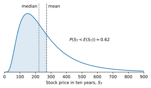
The log price grows at the rate \mu - \frac{1}{2} \sigma^{2}, and the expected price at the faster rate \mu. The gap comes from the right skew of the lognormal distribution. The median is the price at which the log price is at its mean, \text{Median}(S_{T}) = S_{0} e^{\left(\mu - \frac{1}{2} \sigma^{2}\right) T} < S_{0} e^{\mu T} = \operatorname{E}(S_{T}). \tag{5} A few paths that end very high pull the mean above what a typical path achieves, as Figure 1 shows. The realized growth rate \frac{1}{T} \ln(S_{T} / S_{0}) converges to \mu - \frac{1}{2} \sigma^{2} as T \to \infty, so this is the rate a long-term holder typically earns, while \mu is the rate at which wealth grows on average across all paths. The price ends below its mean when \sigma B_{T} < \frac{1}{2} \sigma^{2} T, which has probability \operatorname{P}\left(Z < \frac{1}{2} \sigma \sqrt{T}\right) > \frac{1}{2}.

Figure 1: Density of the stock price in ten years for S_{0} = 100, \mu = 0.10 and \sigma = 0.20. The dotted line marks the median S_{0} e^{(\mu - \frac{1}{2} \sigma^{2}) T} = 221.4 and the dashed line the mean S_{0} e^{\mu T} = 271.8.

Functions of the Stock Price

The price of a derivative depends on the stock price and time, X_{t} = f(S_{t}, t). Substituting (1) and (\mathop{}\!\mathrm{d}S_{t})^{2} = \sigma^{2} S_{t}^{2} \mathop{}\!\mathrm{d}t into Itô’s lemma gives \mathop{}\!\mathrm{d}X_{t} = \left(\mu S_{t} X_{S} + \frac{1}{2} \sigma^{2} S_{t}^{2} X_{SS} + \frac{\partial f}{\partial t}\right) \mathop{}\!\mathrm{d}t+ \sigma S_{t} X_{S} \mathop{}\!\mathrm{d}B_{t}, \tag{6} with X_{S} = \partial f / \partial S and X_{SS} = \partial^{2} f / \partial S^{2}. The function is driven by the same Brownian motion as the stock, with a volatility set by its sensitivity X_{S}. This common risk is what lets an option be replicated with the stock. For a claim maturing at T it is convenient to use the time to maturity \tau = T - t, and since \partial f / \partial t = -X_{\tau}, \mathop{}\!\mathrm{d}X = X_{S} \mathop{}\!\mathrm{d}S + \frac{1}{2} X_{SS} (\mathop{}\!\mathrm{d}S)^{2} - X_{\tau} \mathop{}\!\mathrm{d}t.

A power of a GBM is again a GBM. For X_{t} = S_{t}^{a}, \frac{\mathop{}\!\mathrm{d}X_{t}}{X_{t}} = \left(a \mu + \tfrac{1}{2} a (a - 1) \sigma^{2}\right) \mathop{}\!\mathrm{d}t+ a \sigma \mathop{}\!\mathrm{d}B_{t}. \tag{7} With a = -1 this explains Siegel’s paradox: if S_{t} is the dollar price of a euro, the euro price of a dollar, 1 / S_{t}, has expected rate of change -\mu + \sigma^{2}, so for 0 < \mu < \sigma^{2} each currency is expected to appreciate against the other.

Practice Problems

1. A broad stock index follows a GBM with an expected return of \mu = 9\% per year and a volatility of \sigma = 20\% per year.

   1. Compute the probability that a buy-and-hold investor in the index loses money over one year, and over 25 years.
   2. Compute the probability that the index at least doubles over ten years, and compare it with the expected value of S_{10} / S_{0}.

2. An investor puts $1 million into one of two funds and holds it for 20 years. Fund A has \mu = 10\% and \sigma = 30\%, and fund B has \mu = 8\% and \sigma = 15\%, both per year.

   1. For each fund, compute the expected value and the median value of the investment after 20 years.
   2. Which fund offers the higher expected return, and which the higher long-run realized growth rate? Explain the difference.
   3. Compute the probability that the investment in fund A ends below the median value of the investment in fund B.

3. A stock follows a GBM with \mu = 6\% and \sigma = 30\% per year, and consider X_{t} = S_{t}^{a} for a constant a.

   1. Use (6) to derive the expected return and the volatility of X_{t}.
   2. Find the value a \neq 0 for which X_{t} has zero drift.

4. The dollar price of one euro, S_{t}, follows a GBM with \mu = 1\% and \sigma = 8\% per year.

   1. Compute the expected rate of change of the euro price of one dollar, 1 / S_{t}, and check whether the two expected rates of change agree on which currency is expected to appreciate.
   2. For which values of \mu, given \sigma = 8\%, is each currency expected to appreciate against the other?
   3. Compute the drift of \ln S_{t} and of \ln(1 / S_{t}), and explain why the log changes do not produce a paradox.