import numpy as np
import matplotlib.pyplot as plt
from scipy.optimize import minimize
import yfinance as yf
import warnings
warnings.simplefilter(action='ignore', category=FutureWarning)
def f(x):
return x**2 - 10*x + 6
x = np.linspace(-2, 12, 100)
plt.plot(x, f(x))
res_left_start = minimize(f, [-100])
res_right_start = minimize(f, [100])Optimization in Python
Minimizing Functions
Main logic for the topic:
Machine learning is fundamentally an optimization problem: we choose parameters to minimize a loss (or maximize an objective).
Minimizing f(x) is equivalent to maximizing -f(x).
Minimization and root-finding are closely connected: solving f(x)=0 can be written as minimizing f(x)^2.
A regression can be estimated directly (“by hand”) as an optimization of squared errors, which is often useful when you want custom or more robust objective functions.
Example: 
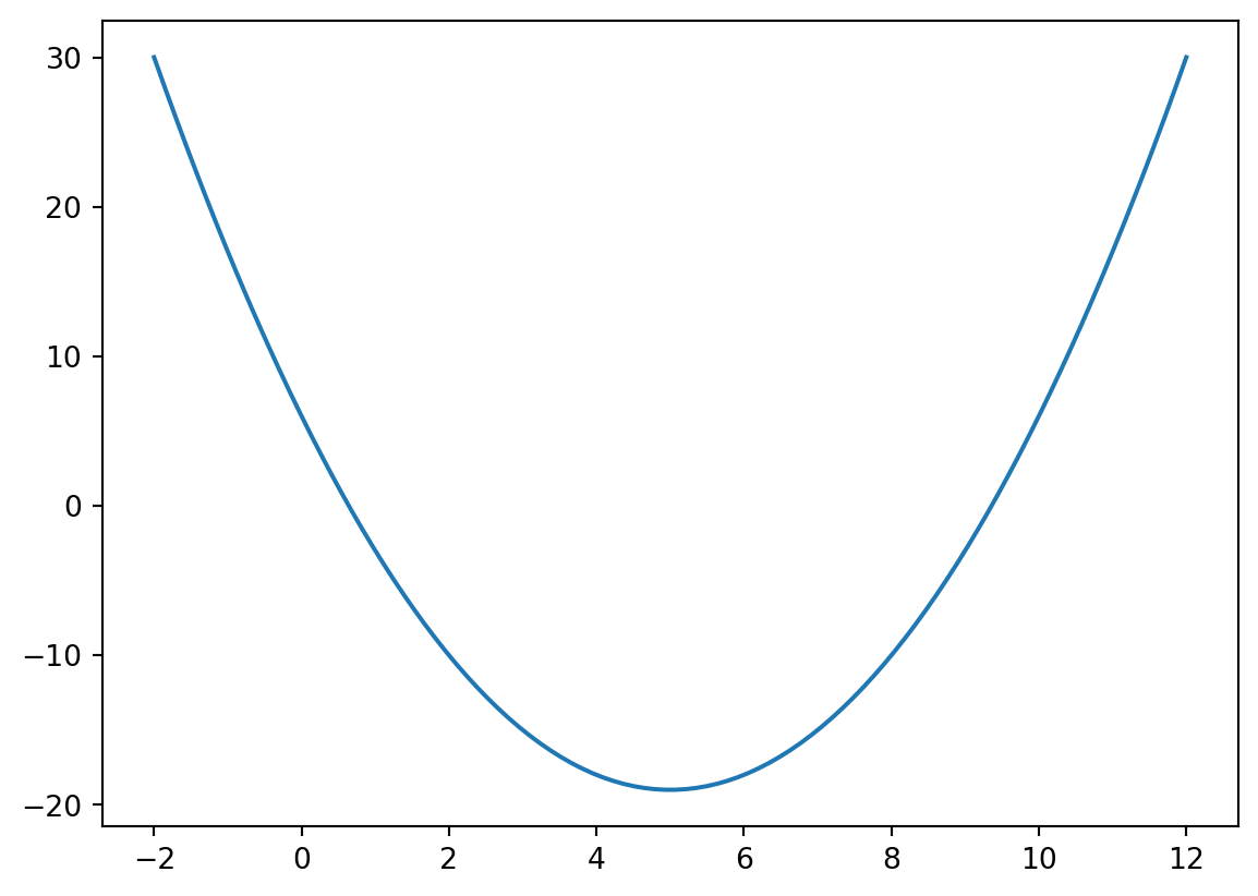
f(x) = x^2 - 10x + 6.
This simple convex function is only used to show how
minimizeworks from different starting values.
Key result:
- From start
-100, optimizer converges to x^*=5.0. - From start
100, optimizer converges to x^*=5.0. - Minimum objective value is f(x^*)=-19.0.
- In the full output objects (
res_left_startandres_right_start),.xis the optimizer solution,.funis the objective value at the solution, and.successreports convergence status.
Root-Finding via Minimization
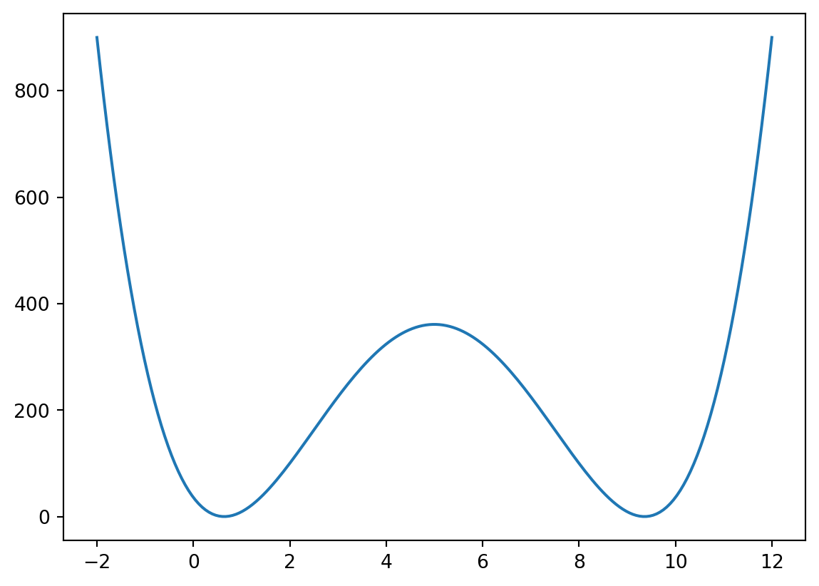
One optimization-based way to find roots of f(x) is to minimize: g(x) = f(x)^2. If f(x)=0, then g(x)=0.
Why this works:
- A square is always nonnegative, so g(x) \ge 0 for every x.
- The minimum possible value of g(x) is therefore 0.
- We get g(x)=0 exactly when f(x)=0, so if a root exists, any global minimizer with objective value 0 is a root.
This approach is useful as a unifying optimization view. In practice, dedicated root-finding methods can be more efficient when their assumptions are satisfied.
def g(x):
return f(x)**2
x = np.linspace(-2, 12, 200)
plt.plot(x, g(x))
res_root_1 = minimize(g, [-2])
res_root_2 = minimize(g, [12])Key result:
- Root near left start: x \approx 0.64.
- Root near right start: x \approx 9.36.
Regression as an Optimization Problem
Estimate a factor model by minimizing squared errors: r_A = \alpha + \beta r_M + e, \text{SSE} = \sum_i (r_{A,i} - \alpha - \beta r_{M,i})^2.
Interpretation:
- Standard OLS is exactly this minimization problem under squared error loss.
- In machine-learning language, this is empirical risk minimization.
- The same framework extends naturally to robust losses (for example absolute loss or Huber loss), regularization, and constraints.
- Scope note: this notebook focuses on in-sample fitting (training) of the objective; it does not perform an out-of-sample backtest.
df = (
yf.download(['MSFT', 'SPY', 'QQQ'], progress=False, start='2000-01-01')['Close']
.resample('ME')
.last()
.pct_change()
.dropna()
)
def mse(theta, dep, ind):
a, b = theta
return np.sum((dep - a - b*ind)**2)
res_base = minimize(mse, [0, 0], args=(df.MSFT, df.SPY))
print(res_base) message: Optimization terminated successfully.
success: True
status: 0
fun: 1.2356241966423969
x: [ 3.011e-03 1.113e+00]
nit: 3
jac: [ 1.490e-08 -5.960e-08]
hess_inv: [[ 1.646e-03 -6.389e-03]
[-6.389e-03 8.457e-01]]
nfev: 18
njev: 6
Extended Models: Result Comparison
The full notebook evaluates two extensions:
- Model 1: add polynomial powers of market return.
- Model 2: add QQQ plus interaction/quadratic terms.
def mse1(theta, dep, ind):
a, b1, b2, b3, b4, b5 = theta
fit = a + b1*ind + b2*ind**2 + b3*ind**3 + b4*ind**4 + b5*ind**5
return np.sum((dep - fit)**2)
def mse2(theta, dep, ind1, ind2):
a, b1, b2, b3, b4, b5 = theta
fit = a + b1*ind1 + b2*ind2 + b3*ind1*ind2 + b4*ind1**2 + b5*ind2**2
return np.sum((dep - fit)**2)
res_poly = minimize(mse1, [0, 0, 0, 0, 0, 0], args=(df.MSFT, df.SPY))
res_two_factor = minimize(mse2, [0, 0, 0, 0, 0, 0], args=(df.MSFT, df.SPY, df.QQQ))
print(f"Base model SSE: {res_base.fun:.4f}")
print(f"Polynomial model SSE: {res_poly.fun:.4f}")
print(f"Two-factor model SSE: {res_two_factor.fun:.4f}")Base model SSE: 1.2356
Polynomial model SSE: 1.2205
Two-factor model SSE: 1.0486
Key results:
- Adding higher SPY powers (Model 1) barely reduces SSE relative to the base model.
- Adding QQQ with interaction and quadratic terms (Model 2) achieves a meaningful in-sample SSE reduction.
Some Final Notes
scipy.optimize.minimizehas many options (method choice, tolerances, constraints, bounds) that are useful in advanced problems.- For standard linear regression workflows,
statsmodelsis usually faster and offers richer inference output. - The optimization approach is still valuable because it extends naturally to nonlinear, constrained, or custom-loss estimation settings.

