import numpy as np
import pandas as pd
import yfinance as yf
import matplotlib.pyplot as plt
import seaborn as sns
import statsmodels.formula.api as smf
import warnings

warnings.simplefilter(action='ignore', category=FutureWarning)

coins = ['BTC-USD','ETH-USD','LTC-USD','XRP-USD','DOGE-USD','BCH-USD','XLM-USD']

df = (
    yf.download(coins, start='2015-01-01', progress=False)['Close']
      .resample('ME')
      .last()
      .pct_change()
      .dropna()
)
df.columns = [c.replace('-USD','') for c in df.columns]A Market Index for Cryptocurrencies
Introduction
Main purpose in this notebook:
- Apply what we just learned about model fitting and interpretation in a real finance setting.
- Build a crypto market factor (
MKT) and use regressions to separate common market exposure (beta) from coin-specific risk (R^2 gaps). - Compare crypto-market returns with stock-market returns (
SPY).
Core model: one-factor return decomposition for each coin i. r_i = \alpha_i + \beta_i r_{\text{MKT}} + e_i.
Interpretation:
- r_{\text{MKT}}: common crypto market shock (systematic component).
- \beta_i: sensitivity of coin i to that common shock.
- \alpha_i: average return component not explained by the factor.
- e_i: idiosyncratic component (coin-specific variation).
Why this model is useful:
- It decomposes returns into common risk vs coin-specific risk.
- It gives a compact way to compare coins with two summary statistics:
Betafor sensitivity.- R^2 for fraction of variance explained by the common factor.
Important distinction for interpretation:
- High beta does not necessarily imply high R^2.
- A coin can react strongly to market moves on average (high beta), yet still have large idiosyncratic volatility (low R^2).
Coins in the index:
| Ticker | Coin |
|---|---|
| BTC | Bitcoin |
| ETH | Ethereum |
| BCH | Bitcoin Cash |
| LTC | Litecoin |
| XRP | Ripple |
| DOGE | Dogecoin |
| XLM | Stellar |
Sample period used in the code:
- Monthly returns from January 2015 onward (subject to data availability for each asset).
Building a Crypto Market Index
Factor model used for each coin i: r_i = \alpha_i + \beta_i r_{\text{MKT}} + e_i.
MKT is a fixed-weight crypto index (weights based on market-cap shares).
Modeling choice:
- We use fixed weights for transparency and stability of interpretation.
- With time-varying weights, measured beta can mix true exposure changes with index-reweighting effects.
w_raw = pd.Series({
    'BTC': 57.5,
    'ETH': 11.6,
    'XRP': 3.8,
    'DOGE': 0.7,
    'BCH': 0.4,
    'LTC': 0.2,
    'XLM': 0.2
})

w = w_raw / w_raw.sum()
weights = pd.DataFrame(np.tile(w.values, (len(df.index), 1)), index=df.index, columns=w.index)
df['MKT'] = (weights * df[w.index]).sum(axis=1)
Analyzing the Relationship Between Cryptocurrencies and the Crypto Market Index
First, we benchmark crypto market volatility against equities:
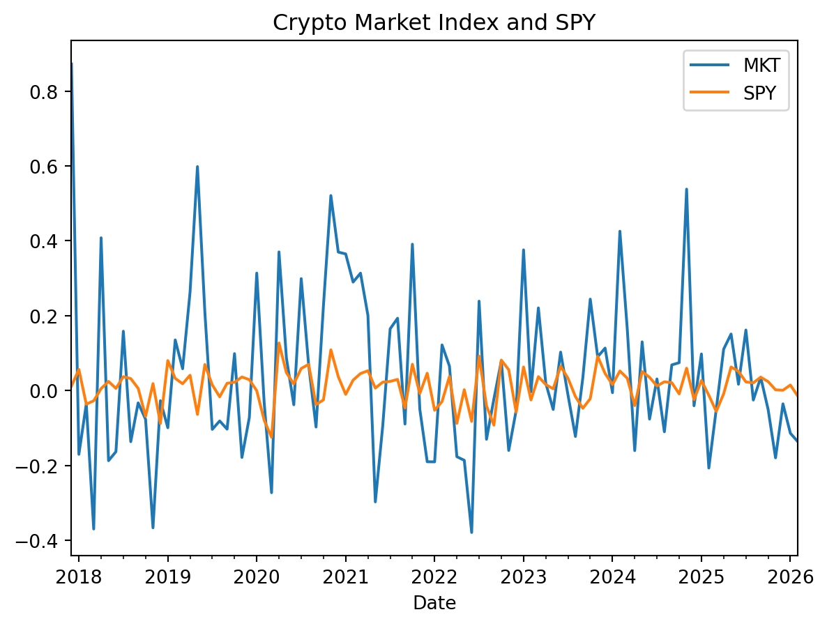
Key results (in this sample):
- The crypto market index is much more volatile than SPY.
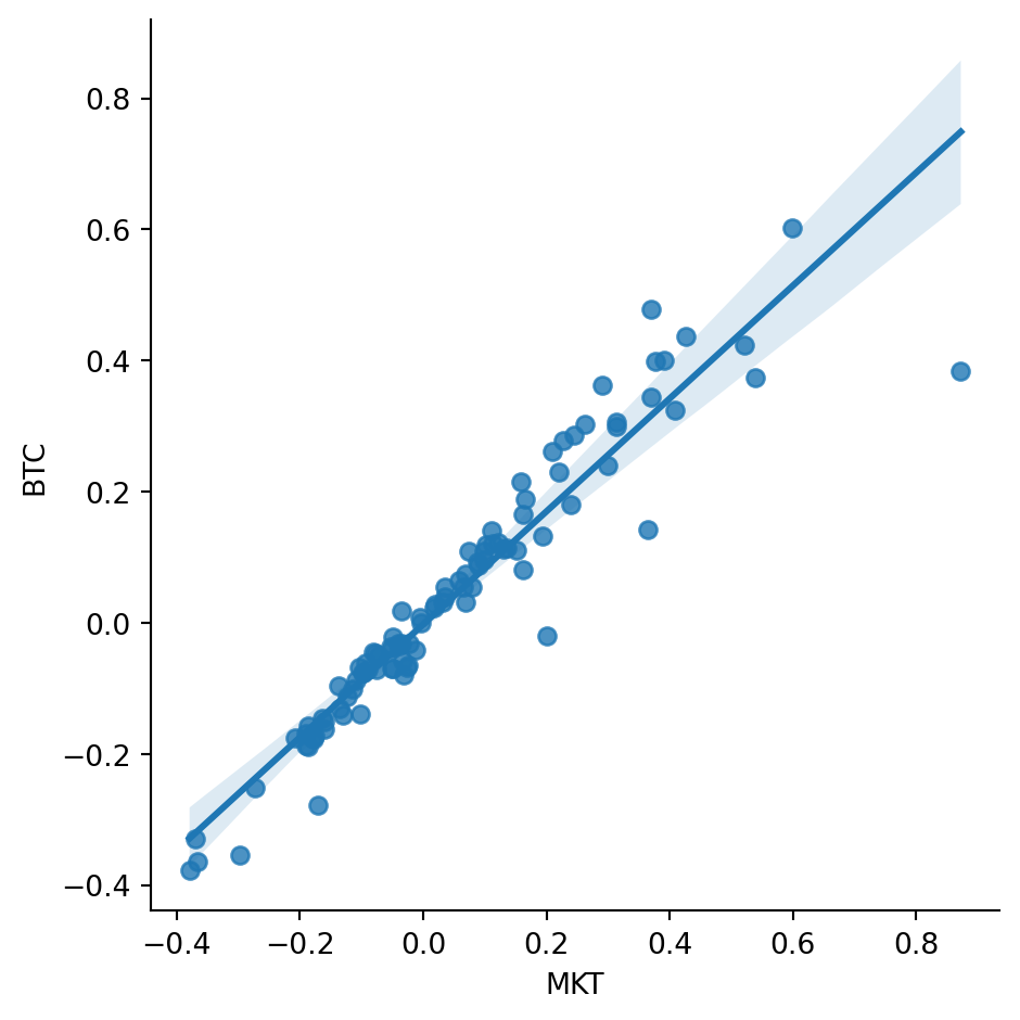
BTC vs MKT
| beta_MKT | p_value(beta=0) | R_squared | |
|---|---|---|---|
| 0 | 0.8612 | 0.0 | 0.9023 |
BTC interpretation:
- BTC has strong positive exposure to the crypto market factor.
- The fit is tight (high R^2), consistent with BTC’s large index weight.
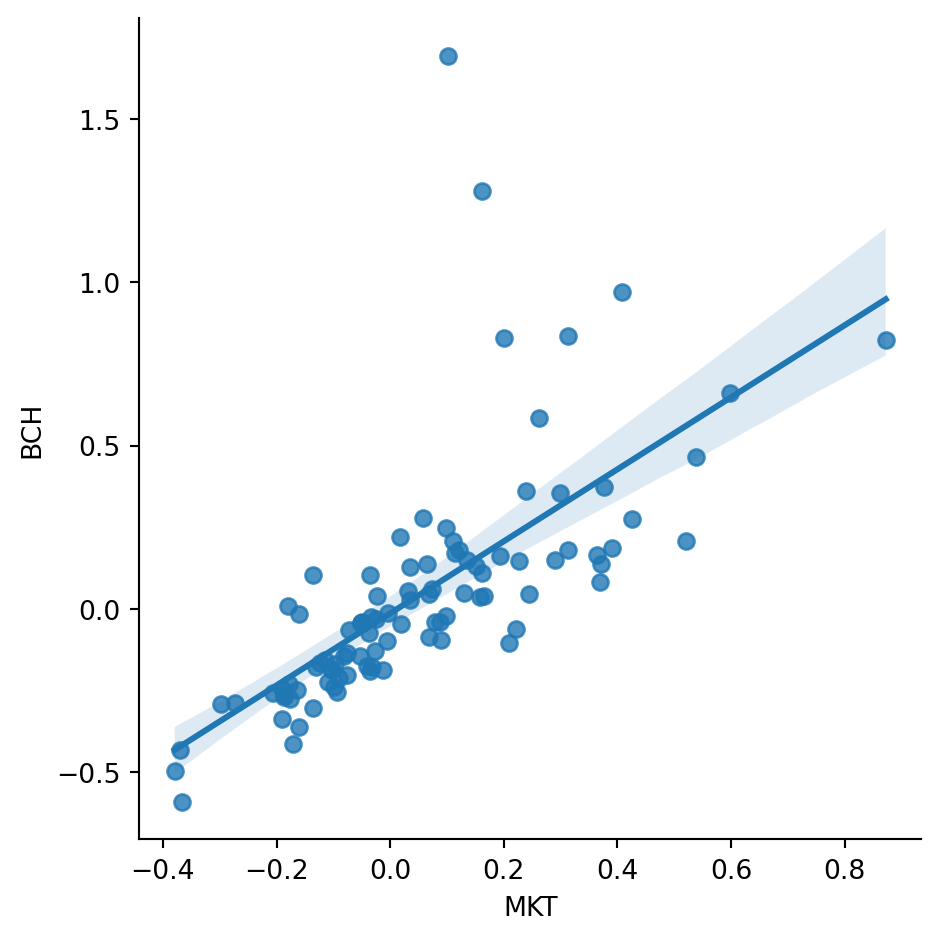
BCH vs MKT
| beta_MKT | p_value(beta=0) | R_squared | |
|---|---|---|---|
| 0 | 1.1018 | 0.0 | 0.4748 |
BCH interpretation:
- BCH still has meaningful market exposure.
- The relationship is noisier than BTC (lower R^2), so more variation is coin-specific.
All Coins on MKT
| Coin | Beta | R-squared | |
|---|---|---|---|
| 7 | MKT | 1.00 | 1.000 |
| 1 | BTC | 0.86 | 0.902 |
| 3 | ETH | 1.08 | 0.721 |
| 4 | LTC | 1.06 | 0.690 |
| 0 | BCH | 1.10 | 0.475 |
| 5 | XLM | 2.07 | 0.433 |
| 6 | XRP | 2.59 | 0.368 |
| 2 | DOGE | 2.13 | 0.229 |
Cross-coin interpretation:
- High beta with low R^2 means strong average market sensitivity but substantial idiosyncratic risk.
- DOGE, XLM, and XRP show relatively high betas but lower R^2, indicating strong average market sensitivity alongside substantial coin-specific risk.
- Sanity check: the
MKTrow should show beta =1 and R^2=1 when regressingMKTon itself.
Statistical reading guide:
- Testing \beta=0: asks whether market exposure is statistically different from zero.
- Confidence intervals: show plausible ranges for true exposure.
- Economic significance (beta size) and statistical significance (p-value) are related but distinct.
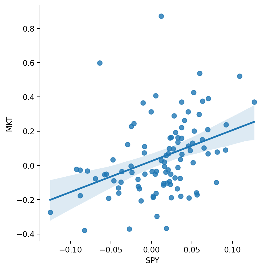
Crypto Market Index vs. Stock Market
Scatter relationship:
| beta_SPY | p_value(beta_SPY=0) | p_value(beta_SPY=1) | R_squared | |
|---|---|---|---|---|
| 0 | 1.8102 | 0.0001 | 0.0682 | 0.1489 |
Key results (in this sample):
SPYloading inMKT ~ SPYis positive and statistically significant (reject \beta_{SPY}=0).- Testing \beta_{SPY}=1: at the 5% level we fail to reject equality to 1, though the result is borderline at the 10% level.
Economic interpretation:
- A positive, significant SPY loading indicates directional co-movement between crypto and equities.
- But R^2 is still crucial: co-movement can be significant while a large share of crypto variation remains unexplained by equities.
Takeaways
- This notebook applies the same regression logic from previous notes to a realistic asset-pricing use case.
Betameasures average market sensitivity; R^2 measures how much variation the market factor explains.- Crypto and equities co-move, but a large share of crypto risk remains crypto-specific.
- Scope note: this notebook is an in-sample modeling exercise (fit and interpretation), not a trading backtest.