import numpy as np
import pandas as pd
import matplotlib.pyplot as plt
from scipy.optimize import minimize
import yfinance as yf

import warnings
warnings.simplefilter(action='ignore', category=FutureWarning)

TRAIN_END = '2024-12-31'
TEST_START = '2025-01-01'
MIN_MONTHS = 36
N_TOP = 50Minimum Variance Portfolio
Introduction
Main purpose in this notebook:
- Estimate a minimum-variance equity portfolio in-sample (2020–2024).
- Compare constrained (
No Short) and unconstrained (Short Allowed) solutions. - Evaluate out-of-sample cumulative performance from January 2025 onward.
What we are trying to do, conceptually:
- We are not forecasting returns directly.
- We are choosing weights to minimize estimated portfolio variance, using historical covariance structure.
- Then we test whether that low-variance construction produces better realized risk-adjusted outcomes out-of-sample.
Setup
Build the Universe and Returns Panel
mcap = pd.read_csv('./stocks_mktcap_202412.csv')
tickers = mcap['TICKER'].unique().tolist()

rets = (yf
      .download(tickers, start='2020-01-01', progress=False)['Close']
      .resample('ME')
      .last()
      .pct_change()
      .dropna(how='all'))

train_rets = rets.loc[:TRAIN_END]
valid = train_rets.count() >= MIN_MONTHS
eligible = mcap.loc[mcap['TICKER'].isin(train_rets.columns[valid])]

top = (eligible.sort_values('MCAP', ascending=False)
              .head(N_TOP)['TICKER']
              .tolist())

df = rets[top]
train = df.loc[:TRAIN_END]
test = df.loc[TEST_START:].dropna()
Data-design note:
- Eligibility is determined using only the training window (
train_rets) to avoid look-ahead bias. - The test sample starts in January 2025 and is not used to estimate weights.
- The
dropna()call in the test panel keeps only months with complete returns for all selected stocks, so the effective out-of-sample window can be shorter than the calendar window.
Estimate Minimum Variance Weights
Optimization problem: \min_{\mathbf{w}}\; \mathbf{w}'\Sigma\mathbf{w} \quad\text{s.t.}\quad \mathbf{1}'\mathbf{w}=1.
Estimation logic:
- Estimate the covariance matrix \Sigma from the training sample.
- Solve the constrained optimization (
No Short). - Solve the unconstrained optimization (
Short Allowed). - Keep weights fixed and evaluate both choices on the test window.
Constraint interpretation:
No Shortimposes 0 \le w_i \le 1, which shrinks extreme positions.Short Allowedremoves box constraints, allowing levered long-short exposures.- In finite samples, the unconstrained solution can overreact to covariance estimation noise.
n = train.shape[1]
cov = train.cov().values
w0 = np.ones(n) / n
objective = lambda w: w @ cov @ w
sum_to_one = {'type': 'eq', 'fun': lambda w: w.sum() - 1}

res = minimize(objective, w0, method='SLSQP', bounds=[(0, 1)] * n, constraints=[sum_to_one])
res_short = minimize(objective, w0, method='SLSQP', constraints=[sum_to_one])
Inspect Estimated Weights
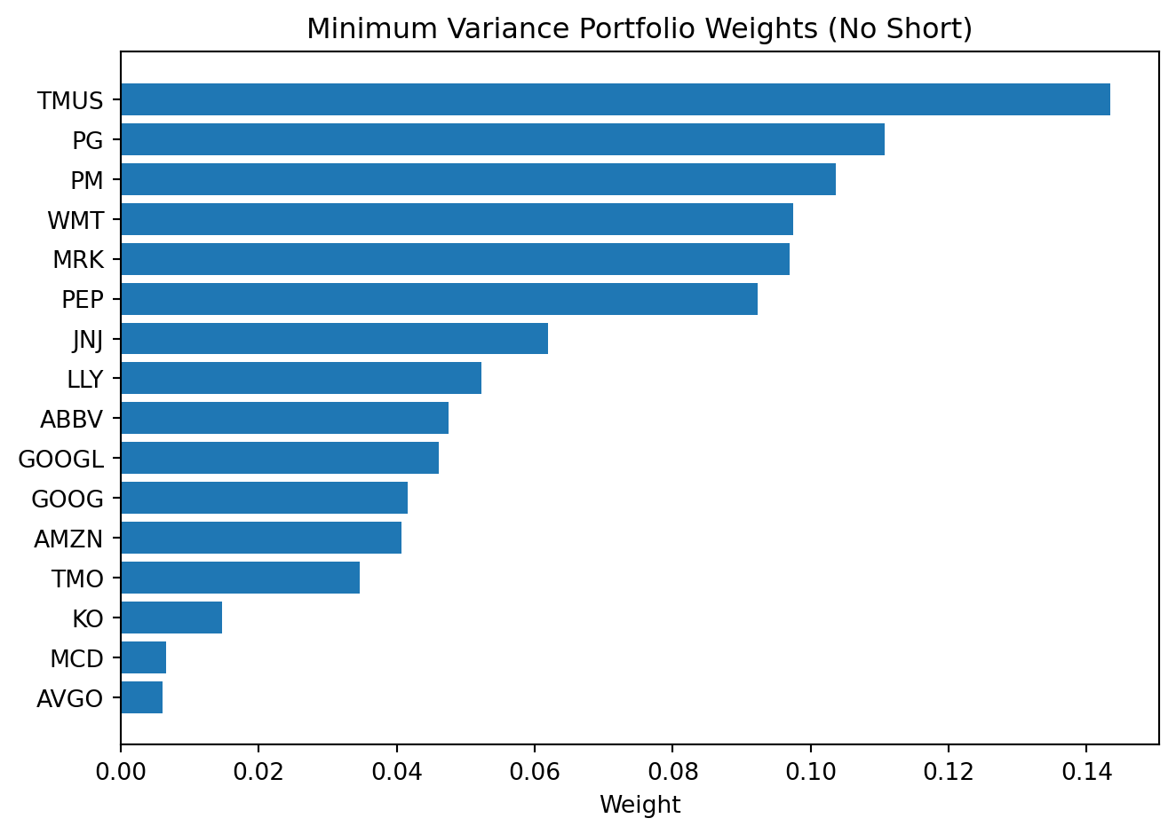
Display filter for the no-short plot:
- Show only holdings with
WEIGHT > 0.5%. - This removes tiny allocations so the chart is readable.
Display filter for the short-allowed plot:
- Show only positions with
abs(WEIGHT) > 6%. - This keeps only economically large long/short positions; smaller offsets are hidden for clarity.
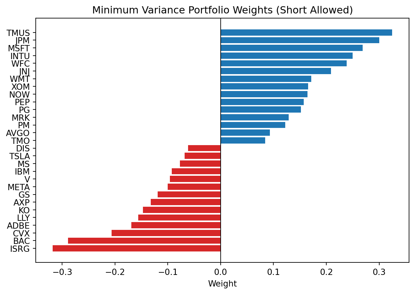
Interpretation:
No Shorttends to produce sparser, more stable allocations.Short Allowedoften creates more extreme positive/negative positions.- Those extremes can look optimal in-sample but may be fragile out-of-sample.
Backtest: January 2025 Onward
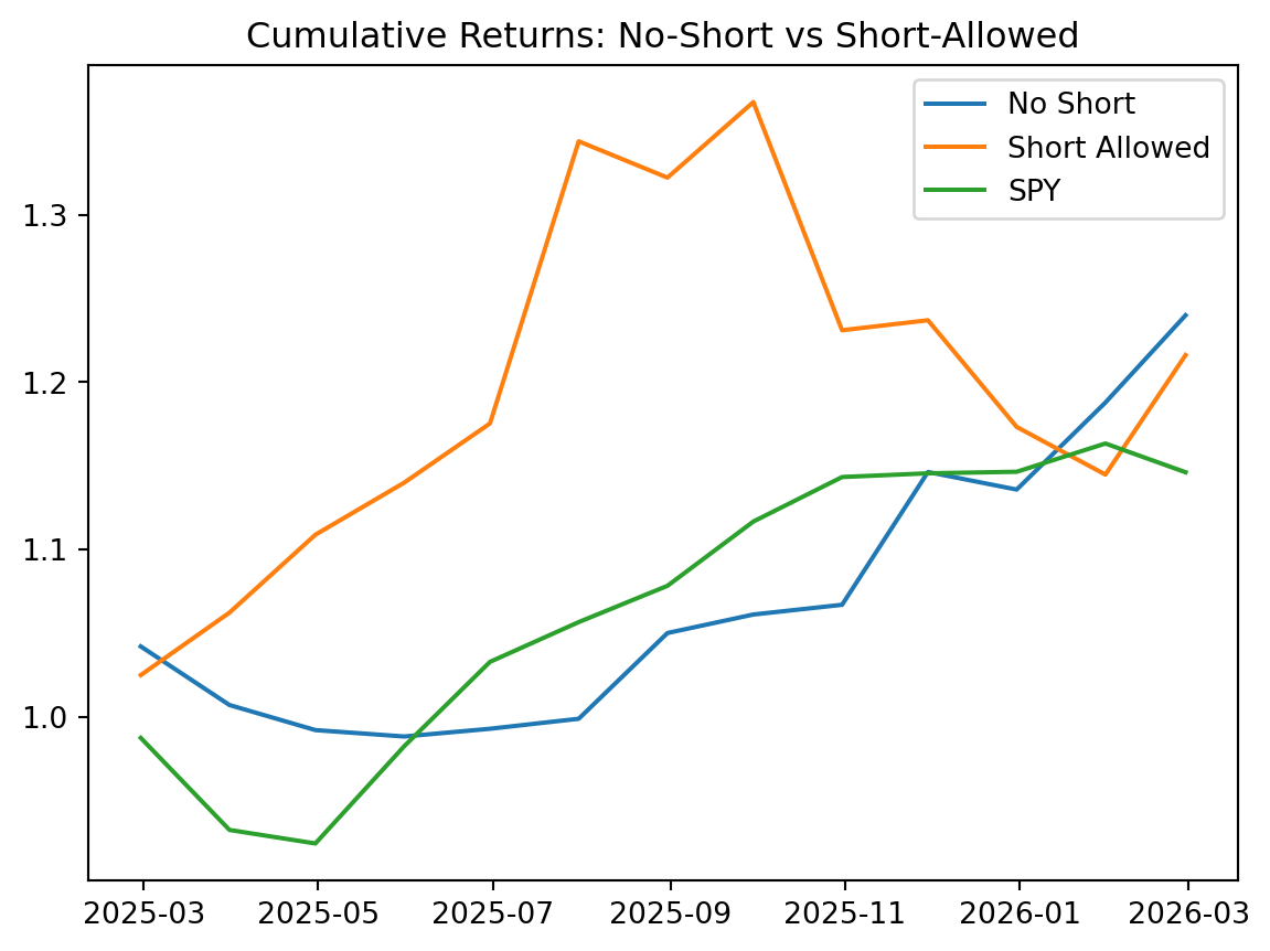
Key result in the notebook sample:
No ShortoutperformsShort AllowedandSPYin this out-of-sample window.- This is consistent with Jagannathan and Ma (2003): in large portfolios, no-short constraints reduce the impact of covariance estimation error by shrinking extreme positions.
- This comparison is based on one realized period, so it is evidence for this sample, not a universal dominance result.
Jagannathan, Ravi, and Tongshu Ma. 2003. “Risk Reduction in Large Portfolios: Why Imposing the Wrong Constraints Helps.” Journal of Finance 58 (4): 1651–83.
How to read the backtest plot:
- Relative slope indicates average realized growth rate over the period.
- Drawdown depth indicates realized risk in stressful months.
- If
No Shortshows smoother growth with smaller drawdowns, that is consistent with a regularization effect: the no-short constraint shrinks extreme covariance-driven weights, reducing sensitivity to covariance estimation error.
Takeaways
- Minimum-variance optimization is highly sensitive to covariance estimation and constraints.
- No-short constraints can improve stability and implementation realism.
- The economic objective is better risk-adjusted performance (Sharpe improvement), not alpha generation. In fact, the expected return of the minimum variance portfolio is typically lower than the market’s — the gain comes from reduced volatility, not higher returns.
- When short-selling is allowed, the optimizer can take on large levered positions that are often unrealistic in practice due to transaction costs, liquidity constraints, and risk management policies. The no-short solution is usually easier and cheaper to implement.
- This notebook is a training/evaluation exercise in one sample period, not a universal portfolio rule.