Analyzing Mutual Fund Performance

Mutual Funds

In this summary we analyze the Fidelity Value Fund (ticker: FDVLX) using monthly data from December 1994 to January 2026.

The Augmented Five-Factor Model

R_{i} = a_{i} + b_{i} R_{m} + s_{i} \mathit{SMB} + h_{i} \mathit{HML} + r_{i} \mathit{RMW} + c_{i} \mathit{CMA} + m_{i} \mathit{MOM} + e_{i}, where R_i = r_i - r_f is the fund excess return and R_m = r_m - r_f is the market excess return.

Interpretation:

  • b_i < 1 implies less systematic risk than the market; b_i > 1 implies more.
  • s_i > 0 implies small-cap tilt; s_i < 0 implies large-cap tilt.
  • h_i > 0 implies value tilt; h_i < 0 implies growth tilt.
  • r_i > 0 implies robust-profitability tilt.
  • c_i > 0 implies low-investment tilt.
  • m_i > 0 implies momentum/winner tilt; m_i < 0 implies contrarian/loser tilt.

Data and Model Setup

Estimating the Model

CAPM

results_capm = smf.ols("RETRF ~ RMRF", data=merged).fit()
print(results_capm.summary(slim=True))
                            OLS Regression Results                            
==============================================================================
Dep. Variable:                  RETRF   R-squared:                       0.632
Model:                            OLS   Adj. R-squared:                  0.631
No. Observations:                 372   F-statistic:                     634.4
Covariance Type:            nonrobust   Prob (F-statistic):           3.03e-82
==============================================================================
                 coef    std err          t      P>|t|      [0.025      0.975]
------------------------------------------------------------------------------
Intercept      0.0043      0.002      2.282      0.023       0.001       0.008
RMRF           1.0445      0.041     25.187      0.000       0.963       1.126
==============================================================================

Notes:
[1] Standard Errors assume that the covariance matrix of the errors is correctly specified.

The CAPM alpha is positive (a = 0.0043) and statistically significant at the 5% level (p-value = 0.023), so the fund outperformed the market after adjusting only for market exposure.

Augmented Five-Factor Model + Momentum

results_ff6 = smf.ols("RETRF ~ RMRF + SMB + HML + RMW + CMA + MOM", data=merged).fit()
print(results_ff6.summary(slim=True))
                            OLS Regression Results                            
==============================================================================
Dep. Variable:                  RETRF   R-squared:                       0.760
Model:                            OLS   Adj. R-squared:                  0.756
No. Observations:                 372   F-statistic:                     192.4
Covariance Type:            nonrobust   Prob (F-statistic):          9.25e-110
==============================================================================
                 coef    std err          t      P>|t|      [0.025      0.975]
------------------------------------------------------------------------------
Intercept      0.0027      0.002      1.680      0.094      -0.000       0.006
RMRF           1.0648      0.039     26.989      0.000       0.987       1.142
SMB            0.3163      0.056      5.654      0.000       0.206       0.426
HML            0.3767      0.066      5.691      0.000       0.247       0.507
RMW            0.2921      0.071      4.106      0.000       0.152       0.432
CMA            0.1150      0.094      1.223      0.222      -0.070       0.300
MOM           -0.1049      0.034     -3.062      0.002      -0.172      -0.038
==============================================================================

Notes:
[1] Standard Errors assume that the covariance matrix of the errors is correctly specified.

After controlling for the other factors, the alpha is positive (a = 0.0027) but only marginally significant at the 10% level (p-value = 0.094). In other words, the fund outperformed by 0.27 \times 12 = 3.24\% per year after controlling for systematic factors, though this result is not statistically significant at conventional levels.

Factor Coefficient Significance Interpretation
SMB 0.3163 1% The fund invested in small stocks
HML 0.3767 1% The fund invested in value stocks
RMW 0.2921 1% The fund invested in stocks with strong profitability
CMA 0.1150 Not significant The fund invested in both high and low investment stocks
MOM -0.1049 1% The fund was significantly contrarian by chasing losers

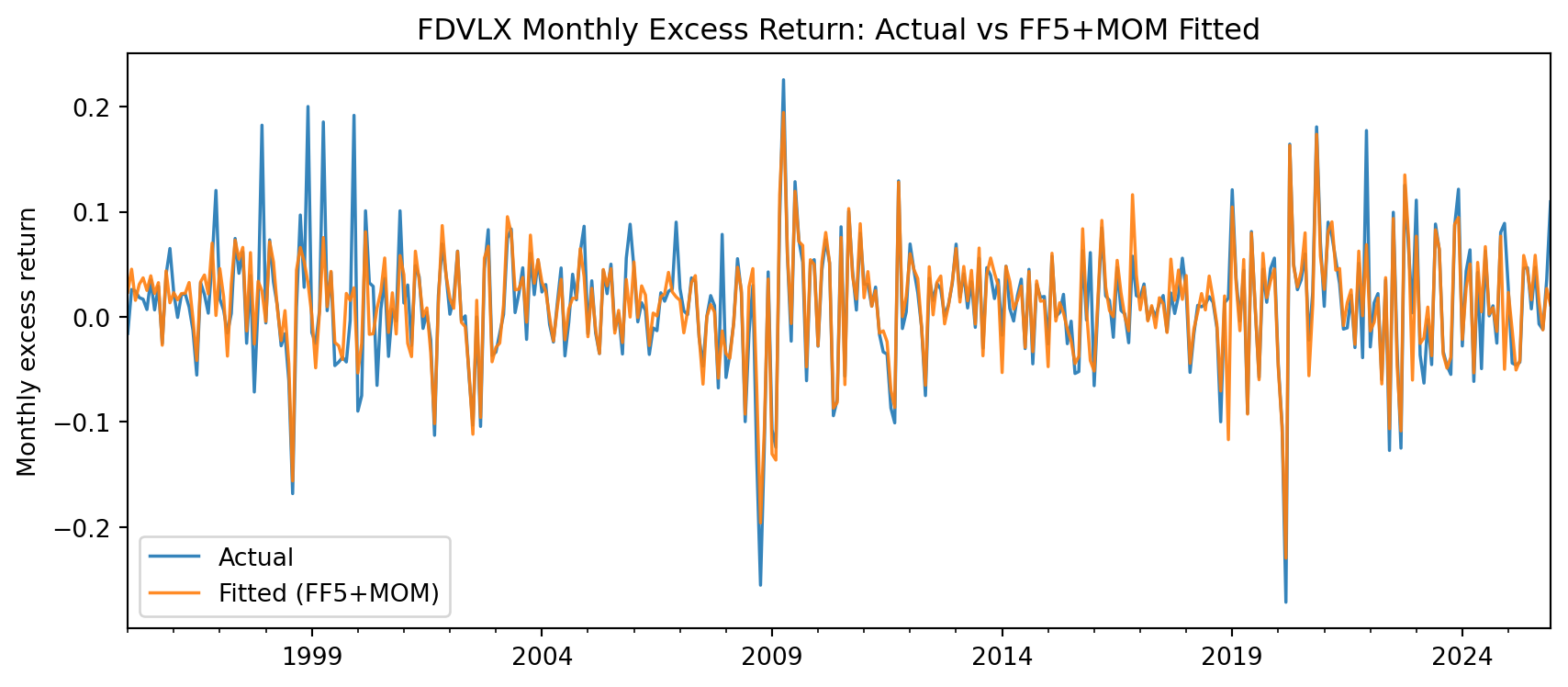
Fit Check (Actual vs Fitted Excess Return)

The next plot compares realized excess returns against fitted values from the augmented model.

fit_df = pd.DataFrame({
    "actual": merged["RETRF"],
    "fitted_ff6": results_ff6.fittedvalues
}).dropna()

ax = fit_df.plot(figsize=(9, 4), lw=1.3, alpha=0.9)
ax.set_title("FDVLX Monthly Excess Return: Actual vs FF5+MOM Fitted")
ax.set_ylabel("Monthly excess return")
ax.set_xlabel("")
ax.legend(["Actual", "Fitted (FF5+MOM)"])
plt.tight_layout()
plt.show()

Economic Interpretation

The results from the regression broadly agree with the fund description. The exposure to SMB is positive, even though Morningstar categorizes the fund as Mid-Cap Value. The fund returns load significantly on HML, which is consistent with the fund being a value fund. The negative exposure to momentum may come from the fact that value firms often have low P/E ratios, which commonly occur after stock price declines. After controlling for all these systematic exposures, alpha is positive but not statistically significant at conventional levels in this sample.

Takeaways

  • Performance evaluation should control for multiple risk factors, not only market beta.
  • Alpha interpretation changes with model specification.
  • Factor regressions are a practical tool for diagnosing how a fund earns returns.