Train MSE: 0.0004
Test  MSE: 0.0004
Test MAE: 0.0163Option Pricing with Neural Networks
Introduction
We generate synthetic option prices from Black-Scholes, train a neural network to learn that pricing map, and evaluate where approximation error is larger or smaller.
The key idea is simple: first define the pricing function analytically, then ask how well a neural network can recover that same function from data alone.
The Black-Scholes Model
Black-Scholes gives a no-arbitrage price for a European call option (exercise only at maturity).
Inputs:
- S: current stock price
- K: strike price
- r: risk-free interest rate
- T: time to maturity (in years)
- \sigma: volatility of stock returns
The call price is C = S N(d_1) - K e^{-rT} N(d_2), d_1=\frac{\ln(S/K)+(r+\frac{1}{2}\sigma^2)T}{\sigma\sqrt{T}}, \qquad d_2=d_1-\sigma\sqrt{T}.
Economic intuition:
- S N(d_1) is the risk-adjusted value of receiving the stock at maturity.
- K e^{-rT} N(d_2) is the present value of paying the strike, adjusted by the risk-neutral exercise probability.
- So the option value is “expected upside from owning stock” minus “expected discounted strike payment.”
Comparative statics from the formula:
- Higher S increases C.
- Higher \sigma usually increases C (more upside convexity).
- Longer maturity T often increases call value (more time for favorable moves).
- Higher r tends to increase call value (discounts the strike more).
From Pricing Model to Learning Problem
Black-Scholes defines a deterministic function from inputs to price. In supervised-learning notation: \mathbf{x}_i = (S_i/K, r_i, T_i, \sigma_i), \quad C_i = f(\mathbf{x}_i), \quad \hat{C}_i = \hat{f}(\mathbf{x}_i;\theta).
Our workflow is:
- Use Black-Scholes to generate targets C_i on a grid of inputs \mathbf{x}_i.
- Train a neural network \hat{f}(\mathbf{x}_i;\theta) to approximate f(\mathbf{x}_i).
- Evaluate out-of-sample error to measure how well \hat{f} recovers the Black-Scholes pricing map.
In the synthetic data we set K=1, so moneyness S/K is numerically equal to S.
Because the targets are generated by Black-Scholes itself, this is an approximation exercise (learning a known nonlinear map), not a test of whether Black-Scholes is correct in real markets.
This is closely related to learning implied volatility: for fixed (S/K, r, T), Black-Scholes gives a one-to-one (monotone) mapping between call price and implied volatility. So learning prices vs learning implied vol differs mainly by a nonlinear transformation.
Neural Networks
A feedforward network approximates nonlinear functions by composing linear maps and nonlinear activations. The model used here is:
- Input layer: 4 features (S/K, r, T, \sigma)
- Hidden layer: 50 neurons with ReLU
- Output layer: 1 value (predicted call price)
With one hidden layer, the prediction is \hat{C}_i = W^{(2)} \phi\left(W^{(1)} \mathbf{x}_i + b^{(1)}\right) + b^{(2)}, \quad \phi(z)=\max(0,z). For this architecture:
- W^{(1)} \in \mathbb{R}^{50 \times 4}, b^{(1)} \in \mathbb{R}^{50}
- W^{(2)} \in \mathbb{R}^{1 \times 50}, b^{(2)} \in \mathbb{R}
ReLU allows piecewise-linear responses, which gives the network enough flexibility to learn the nonlinear Black-Scholes pricing surface.
Training chooses parameters \theta to minimize mean squared error (MSE), \text{MSE} = \frac{1}{N}\sum_{i=1}^{N}(\hat{C}_i-C_i)^2.
Implementation logic:
- Standardize features before training so optimization is numerically stable.
- Split into train/test sets to check held-out fit (generalization).
- Use Adam with mini-batches to update parameters efficiently.
Generating the Training Data
Synthetic design choices:
- Fixed strike at K=1.
- Input grid over (S, r, T, \sigma).
- Small noise added to volatility before generating targets.
Building and Training the Neural Network
We split the sample into a small training set and a large test set. This setup is intentional: it checks whether the network can learn the Black-Scholes surface from limited examples and still generalize well.
The split is random across synthetic observations, so “out-of-sample” here means held-out points from the same data-generating process (not a forward-time forecast exercise).
Before training, we standardize inputs so all features are on comparable scales. This usually makes gradient-based optimization faster and more stable.
The network is trained with mini-batches using Adam to minimize MSE. At each update step, the model:
- Predicts prices for the current batch.
- Computes the pricing error (MSE).
- Backpropagates gradients.
- Updates parameters to reduce future error.
After multiple passes over the training data (epochs), the fitted network represents our learned pricing function \hat{f}.
Evaluating the Model
Evaluation has two goals:
- Fit: Is the model accurate on training data?
- Generalization: Does accuracy remain good on unseen test data?
We report train and test MSE. If test MSE is close to train MSE and both are low, the approximation is accurate without strong overfitting.
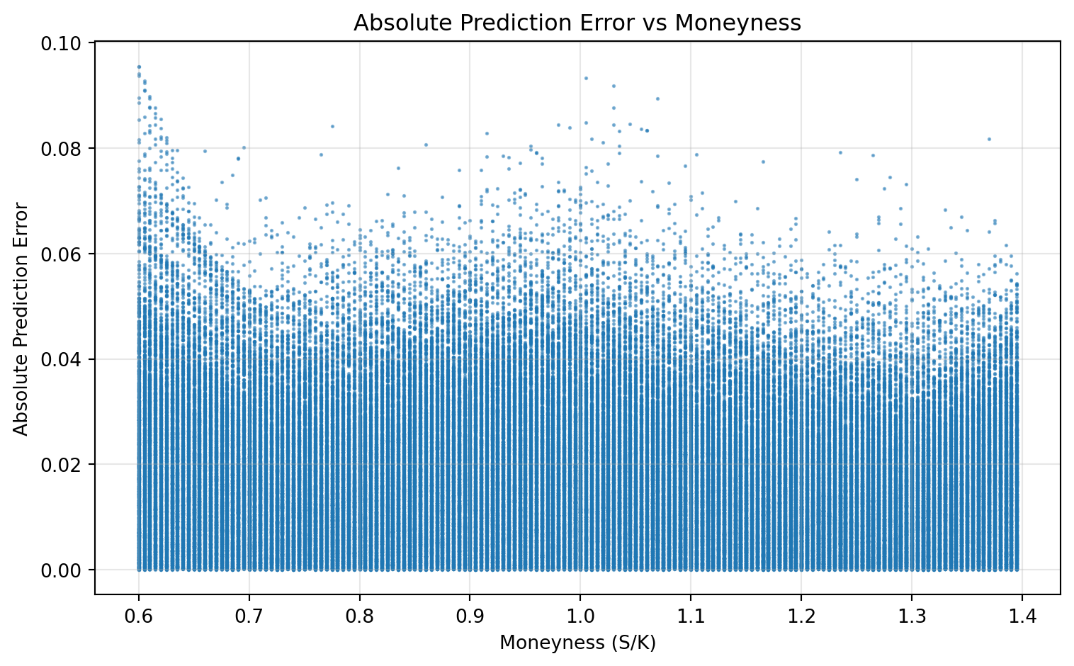
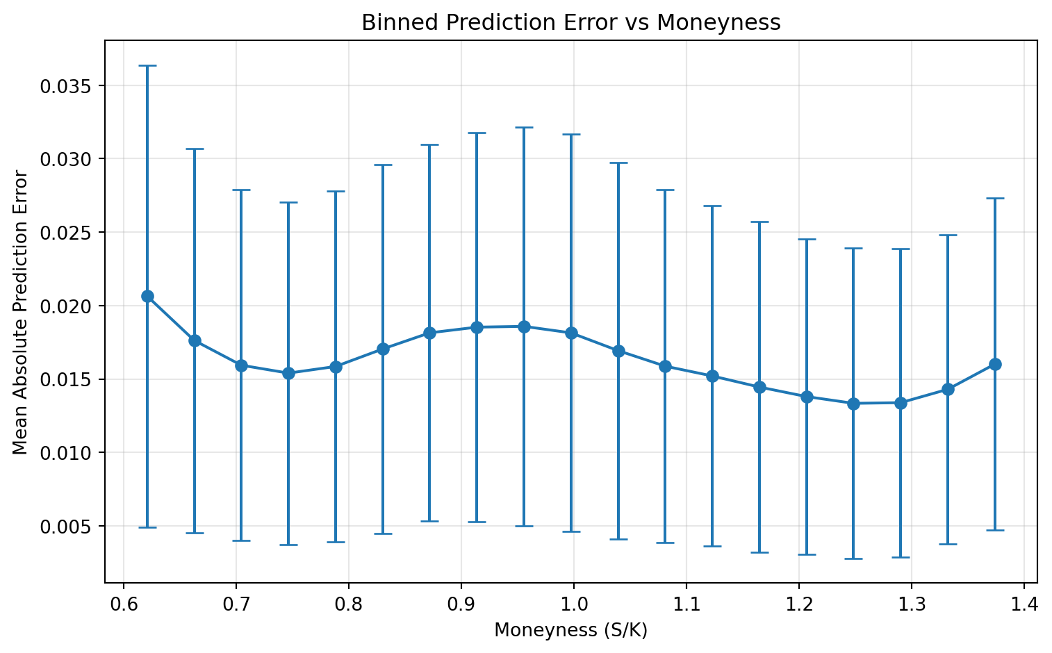
We also compute absolute pricing errors on the test set and analyze them against moneyness. This diagnostic shows where the model is strong or weak across the state space, not only the average error level.
So the evaluation has two layers: global fit (MSE) and local fit (error patterns across moneyness).
Train and test MSE are both low in this synthetic setting, indicating good out-of-sample approximation of Black-Scholes prices.
Main findings:
- The network approximates Black-Scholes prices well in this sample.
- Train and test errors are both low, indicating good generalization under this synthetic setup.
- Error is not uniform across moneyness; diagnostics help identify where fit is weaker.
Takeaways
- Neural networks can learn option-pricing maps as flexible function approximators.
- The framework is still supervised learning: define features, target, loss, optimize.
- Visual diagnostics are as important as headline error metrics.