Blockchain Foundations

Introduction

Main purpose in this notebook:

Build the technical foundation (bytes, hashes, block linkage).
Explain PoW economics and confirmation security.
Connect formal state-process logic to numerical simulation.

Logic of the notebook:

Start with data representation and hashing primitives.
Use those primitives to explain why block linking creates tamper evidence.
Add PoW to show how tamper evidence becomes economically costly to defeat.
Express security as a probabilistic process, then verify key implications numerically.

Bits and Bytes

Core mapping: 10101100_2=\mathrm{AC}_{16}=172_{10}, 256\text{ bits}=32\text{ bytes}=64\text{ hex chars}.

"hello".encode("utf-8").hex()

'68656c6c6f'

Interpretation:

Hashing operates on bytes, not abstract text.
Hex is the compact, readable representation used for hashes and addresses.

Hash Functions

Key properties used in the notebook:

Deterministic output.
Pre-image and collision resistance (computationally hard to break).
Avalanche effect (small input change, large digest change).

import hashlib

def sha256_hex(s):
    return hashlib.sha256(s.encode("utf-8")).hexdigest()

(sha256_hex("hello world"), sha256_hex("Hello World"))

('b94d27b9934d3e08a52e52d7da7dabfac484efe37a5380ee9088f7ace2efcde9',
 'a591a6d40bf420404a011733cfb7b190d62c65bf0bcda32b57b277d9ad9f146e')

Key result:

Even tiny input changes produce drastically different hashes.

Blockchain Mechanics

Core block-linking logic:

Each header includes the previous block hash.
Changing an old block changes its hash and breaks all forward links.
Rewriting history requires re-mining the changed block and all successors.

So hash pointers provide integrity of history, while PoW (next section) provides the cost that enforces that integrity in practice.

Proof of Work, Security, and Incentives

PoW validity condition: \text{hash} < \text{target}.

If hash outputs are approximately uniform over a large space, each nonce attempt is a Bernoulli trial with success probability p.

Leading-zero simplification: p=16^{-N},\qquad \mathbb E[K]=\frac{1}{p}=16^N, where K is the number of tries until first success under an N-leading-zero rule.

Economic interpretation:

Block production is costly; verification is cheap.
Rewards are paid only for accepted blocks.
For most miners, honest behavior is privately optimal.
Security comes from this asymmetry: producing valid alternative history is expensive, checking validity is fast.

Mining Pools

Pool intuition in the notebook:

Solo mining has high payout variance.
Pools smooth payouts by sharing rewards.
Contract design shifts variance between miner and pool (e.g., PPS vs PPLNS).
High concentration can increase coordination/security risk.

State-Process View

Block-time state representation: X_t=(h_{t-1},m_t,\tau_t,T_t), with nonce search until first success K_t=\min\{k:r_{t,k}=1\}.

Confirmation-risk benchmark (attacker share q, honest share p): Q_z= \begin{cases} 1, & p\le q,\\ \left(\frac{q}{p}\right)^z, & p>q, \end{cases} This benchmark implies risk declines exponentially in depth z when q<p.

Interpretation:

Each extra confirmation is additional elapsed time for honest miners to extend the chain.
When honest hash power dominates (p>q), deeper confirmations reduce reversal risk quickly.

Numerical Simulation of Mining

The simulation maps theory to computation:

One trial = one nonce hash attempt.
Success = hash with N leading hex zeros.
Repeating many trials estimates the waiting-time distribution for first success.

import random
import statistics
import time
import pandas as pd
import matplotlib.pyplot as plt


def mine_once_leading_zeros(N: int, max_tries: int = 2_000_000):
    prev_hash = "0" * 64
    merkle_root = sha256_hex(f"tx-set-{random.randint(0, 10**9)}")
    timestamp = int(time.time())
    target_prefix = "0" * N

    for nonce in range(max_tries):
        header = f"{prev_hash}|{merkle_root}|{timestamp}|{nonce}"
        if sha256_hex(header).startswith(target_prefix):
            return nonce + 1
    return None

settings = [{"N": 2, "reps": 200}, {"N": 3, "reps": 120}, {"N": 4, "reps": 40}]
rows = []
for s in settings:
    N, reps = s["N"], s["reps"]
    samples = [mine_once_leading_zeros(N) for _ in range(reps)]
    samples = [x for x in samples if x is not None]
    rows.append({
        "N": N,
        "reps": len(samples),
        "theory_E_tries": 16**N,
        "empirical_mean": round(statistics.mean(samples), 2),
        "empirical_median": round(statistics.median(samples), 2),
    })

df_summary = pd.DataFrame(rows)
df_summary

	N	reps	theory_E_tries	empirical_mean	empirical_median
0	2	200	256	257.17	195.5
1	3	120	4096	4419.64	3656.0
2	4	40	65536	75332.45	40441.0

How to read the table:

theory_E_tries is the benchmark 16^N from the geometric-success model.
empirical_mean should be close to theory with enough repetitions.
empirical_median is typically lower than the mean because waiting-time distributions are right-skewed.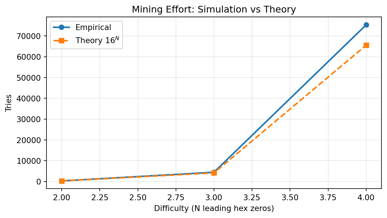

Key result:

Empirical mining effort tracks the geometric benchmark and rises roughly by a factor of 16 per extra leading hex zero.
Small gaps vs theory are expected finite-sample noise from simulation.

Takeaways

Blockchain security combines cryptography, costly block production, and incentives.
PoW is a first-passage search process with exponential difficulty scaling.
Confirmation depth is a risk-management variable with explicit probabilistic interpretation.
The key link is: cryptographic linkage gives tamper evidence, and PoW economics makes tampering costly.