import numpy as np
import pandas as pd
import matplotlib.pyplot as plt
import yfinance as yf
import seaborn as sns

import warnings
warnings.simplefilter(action='ignore', category=FutureWarning)Introduction to Jupyter Notebooks
Introduction
Main purpose in this notebook:
- Introduce the Python workflow used in class.
- Download and transform finance data with
yfinanceandpandas. - Visualize co-movement and volatility differences with simple plots.
Libraries
Data and Returns
df = (yf
      .download(['MSFT', 'SPY'], progress=False, start='2000-01-01')
      .loc[:, 'Close']
      .resample('ME')
      .last()
      .pct_change())
Sample period used in the code:
- Monthly returns from January 2000 onward (subject to data availability).
Return Comparison
df.plot(title='Monthly Returns of MSFT Stock and SPY')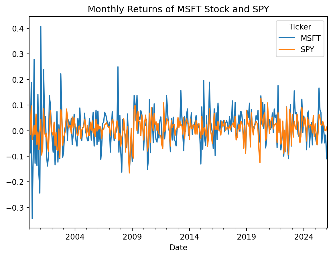
Key result:
SPYreturns are less volatile thanMSFTreturns, consistent with index diversification.
Co-Movement View
sns.lmplot(data=df, x='SPY', y='MSFT')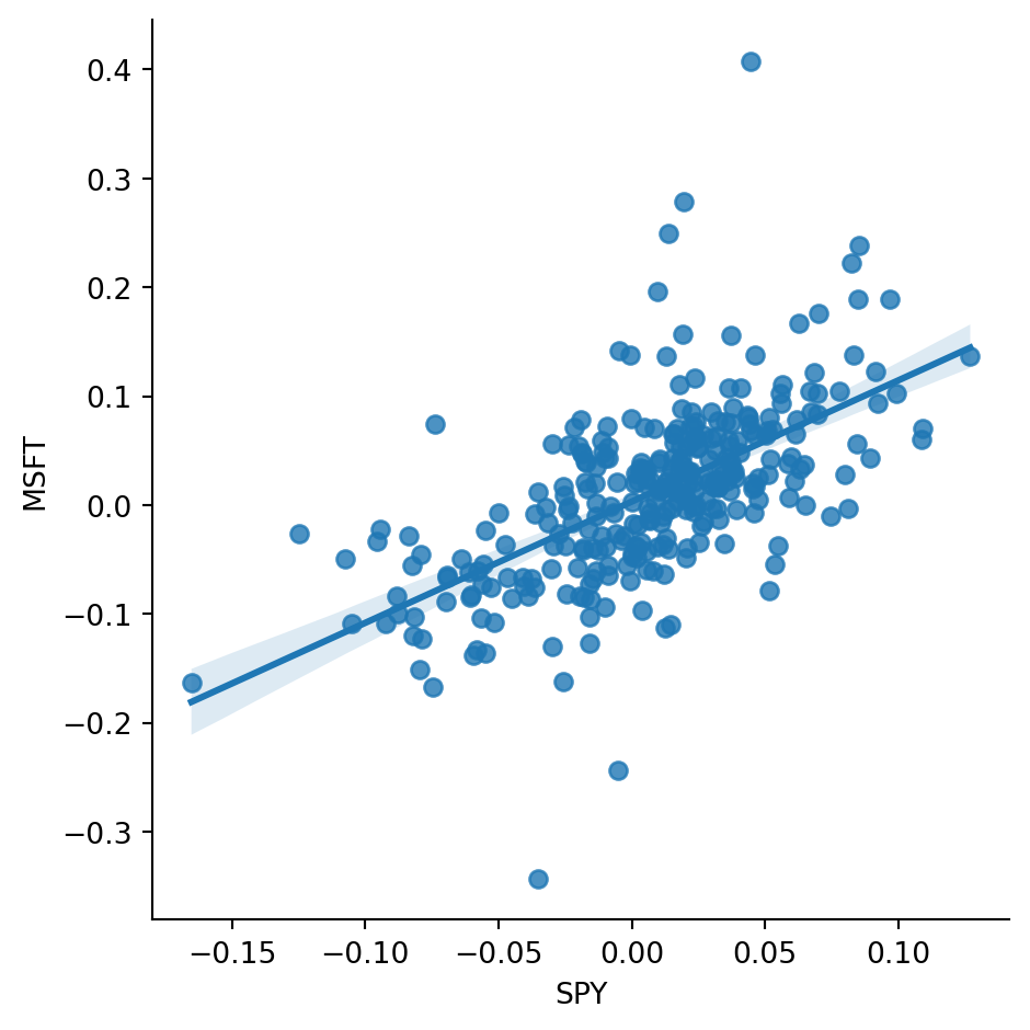
Interpretation:
MSFTandSPYshow clear positive co-movement.- This visual relationship motivates factor-style regressions used later in the course.
Takeaways
yfinance+pandas+ plotting tools are enough for a complete first empirical workflow.- The key steps are: download data, resample, compute returns, and interpret basic diagnostics.
- This notebook is a setup notebook; it introduces tools rather than advanced model testing.