import numpy as np
import matplotlib.pyplot as plt
import pandas as pd
import torch
import torch.nn as nn
from torch.utils.data import DataLoader, TensorDataset
from sklearn.model_selection import train_test_split
from sklearn.preprocessing import StandardScaler
from sklearn.metrics import mean_absolute_error, r2_score
import yfinance as yf

seed = 420
np.random.seed(seed)
torch.manual_seed(seed)
device = torch.device("cuda" if torch.cuda.is_available() else "cpu")

df = pd.read_csv("./108105_2023_C_options_data.csv")
df["date"] = pd.to_datetime(df["date"])

vix = yf.download("^VIX", start="2023-01-01", progress=False, multi_level_index=False)[["Close"]]
vix.columns = ["^VIX"]
df = df.merge(vix, left_on="date", right_index=True, how="left")

cleaned_df = df[["S", "K", "T", "^VIX", "Impl_Vol"]].copy()
cleaned_df = cleaned_df.dropna(subset=["S", "K", "T", "^VIX", "Impl_Vol"])
cleaned_df = cleaned_df[(cleaned_df["Impl_Vol"] < 0.6) & (cleaned_df["T"] > 29) & (cleaned_df["T"] < 681)]
cleaned_df["moneyness"] = cleaned_df["K"] / cleaned_df["S"]
cleaned_df = cleaned_df[cleaned_df["moneyness"] > 0.1]Volatility Surface Modeling with Neural Networks
Introduction
Main purpose in this notebook:
- Apply the same ML fitting logic to real SPX option data.
- Predict implied volatility (IV) from option and market features.
- Evaluate fit quality and compare observed vs predicted IV surfaces.
What we are trying to do, conceptually:
- Here, implied volatility (IV) is the volatility value that, when plugged into an option-pricing model (typically Black-Scholes), matches the market option price.
- So IV is not directly observed like price or volume; it is implied from observed option prices.
- In options markets, IV is not flat; it varies across moneyness and maturity (the IV surface).
- Instead of imposing a rigid parametric shape, we train a neural network to learn the mapping \text{IV} = f\big(\text{moneyness}, T, S, \text{VIX}\big).
- Economically, this is a nonlinear interpolation/extrapolation problem: use historical cross-sections of options to learn a surface that captures level, slope, and curvature patterns in market IV.
- The goal is approximation quality of the observed surface, not structural causal identification.
Scope note:
- This is a modeling workflow focused on approximation quality, not on trading performance.
- Evaluation uses a random held-out test split within the same sample period (not a forward-time backtest).
Data Loading and Preprocessing
Core features used:
- K/S (moneyness)
- T (days to maturity)
- S (spot level)
VIX(market-wide volatility state)
Filter logic:
- Keep observations in a practical IV/maturity region used in class.
- This improves stability and avoids extreme points dominating the fit.
Model Training
Training logic in detail:
- Build supervised-learning inputs and target: X = (K/S,\; T,\; S,\; \text{VIX}),\qquad y = \text{Impl\_Vol}.
- Split into train and test sets so evaluation is on held-out observations relative to the fitted parameters.
- Standardize features using training data only. This avoids scale dominance (for example, raw S vs normalized moneyness) and prevents test-set leakage.
- Use a feedforward neural network with ReLU activations:
- hidden layers transform inputs into nonlinear features,
- final layer maps those features to one scalar prediction (IV).
- Minimize mean squared error (MSE) with Adam: \min_{\theta} \frac{1}{N}\sum_{i=1}^N\big(\hat y_i(\theta)-y_i\big)^2. Backpropagation computes gradients of this objective, and Adam updates parameters iteratively.
- Repeat over epochs:
- each epoch passes through minibatches of training data,
- each minibatch step updates parameters to reduce prediction error.
Training note:
train_size=0.01means only 1% of the sample is used for training (chosen for speed in class/demo settings).- With larger training fractions, fit quality is typically higher but run time increases.
- Using a small train fraction makes this notebook a fast demonstration of workflow; for production modeling, you would usually use much more training data and more formal validation/tuning.
Model Evaluation
Evaluation goal:
- Check not only average error size, but also where errors concentrate and whether the model preserves cross-sectional structure.
- A useful evaluation in options problems is multi-layered:
- scalar metrics (MAE/RMSE/R^2),
- local diagnostics (error vs moneyness),
- calibration diagnostics (predicted vs observed levels).
| MAE | RMSE | R_squared | |
|---|---|---|---|
| 0 | 0.004622 | 0.006905 | 0.96959 |
How to read these metrics:
MAE: average absolute IV error (easy to interpret in IV points).RMSE: penalizes larger errors more than MAE.- R^2: fraction of IV variation explained by the model on the test sample.
Interpretation guide:
- If RMSE is much larger than MAE, a small subset of observations likely has large errors.
- A high R^2 with nontrivial MAE can still occur when the model gets relative ranking right but misses absolute levels in some regions.
- Because IV has regime and moneyness structure, aggregate metrics alone are not enough.
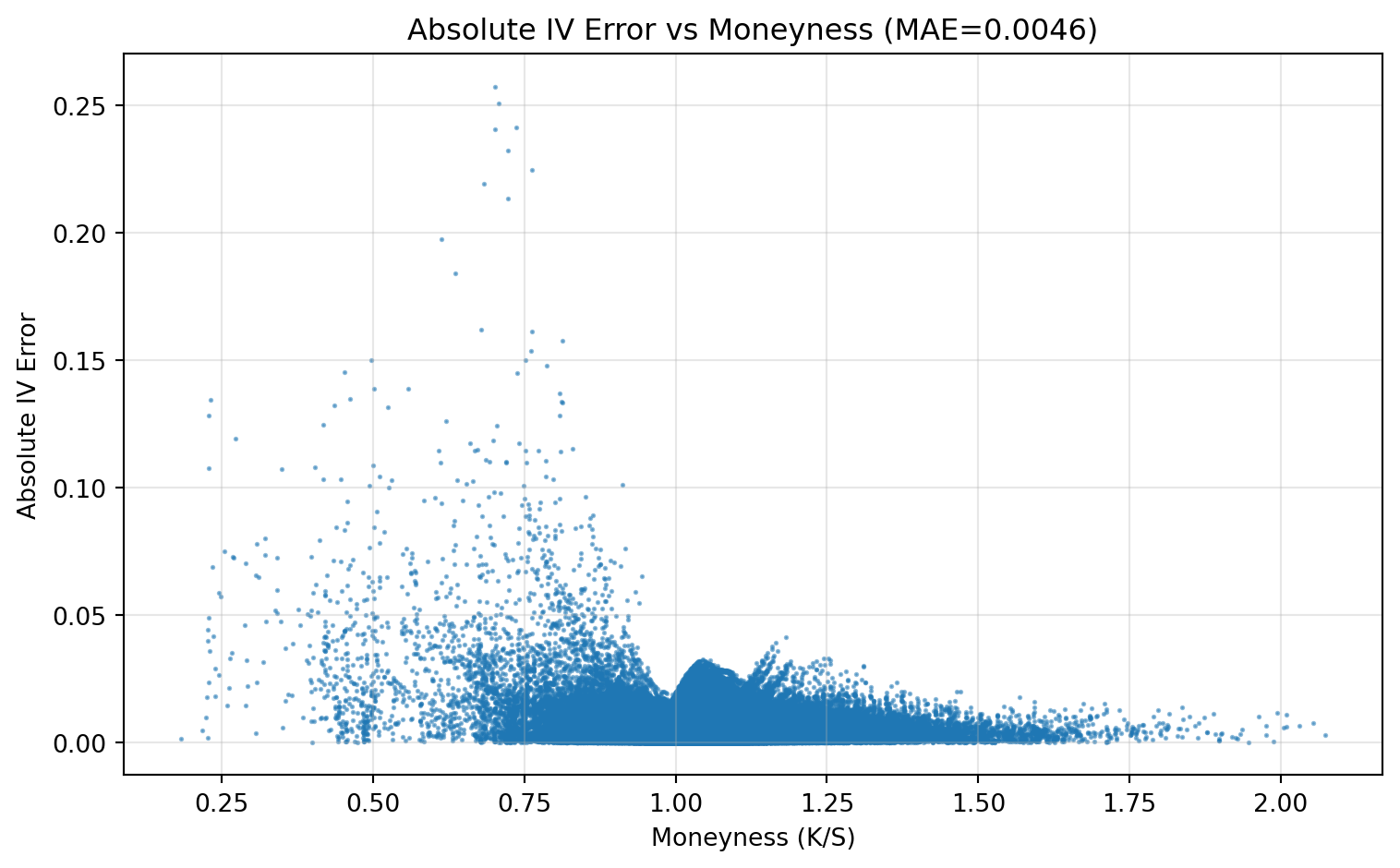
What this plot checks:
- Whether errors are systematically larger in specific moneyness regions (for example deep OTM/ITM).
- Ideally, points should be low and roughly pattern-free; clear bands or slopes indicate model misspecification in that region.
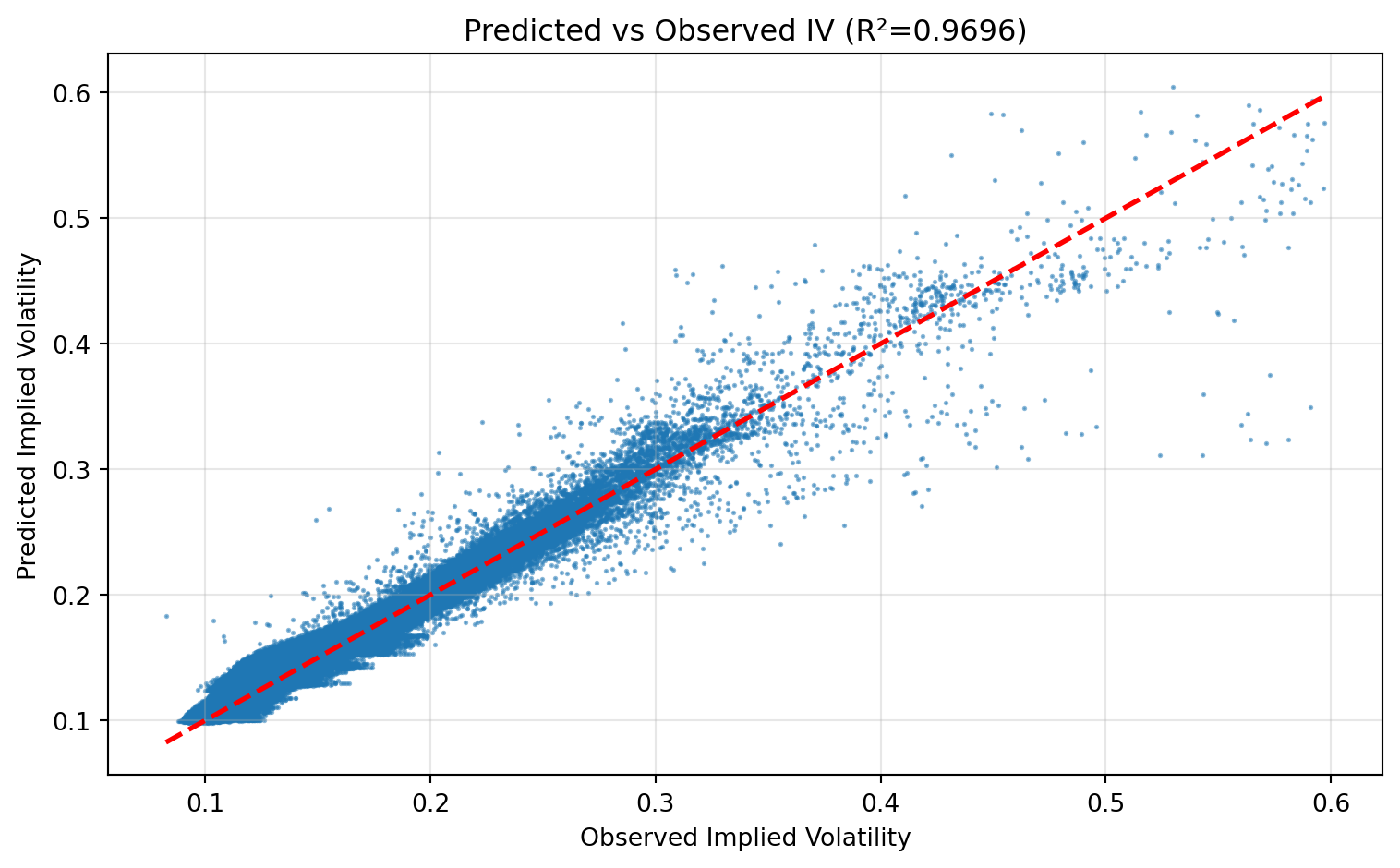
What this plot checks:
- Points near the 45-degree line indicate good calibration.
- Curvature away from the line indicates bias (overprediction/underprediction in parts of the IV range).
- Fan-shaped dispersion indicates heteroskedastic errors (error variance grows with IV level).
Key result:
- The model captures a substantial part of IV variation in this sample, with visible but non-uniform residual error.
Visualizing the Volatility Surface
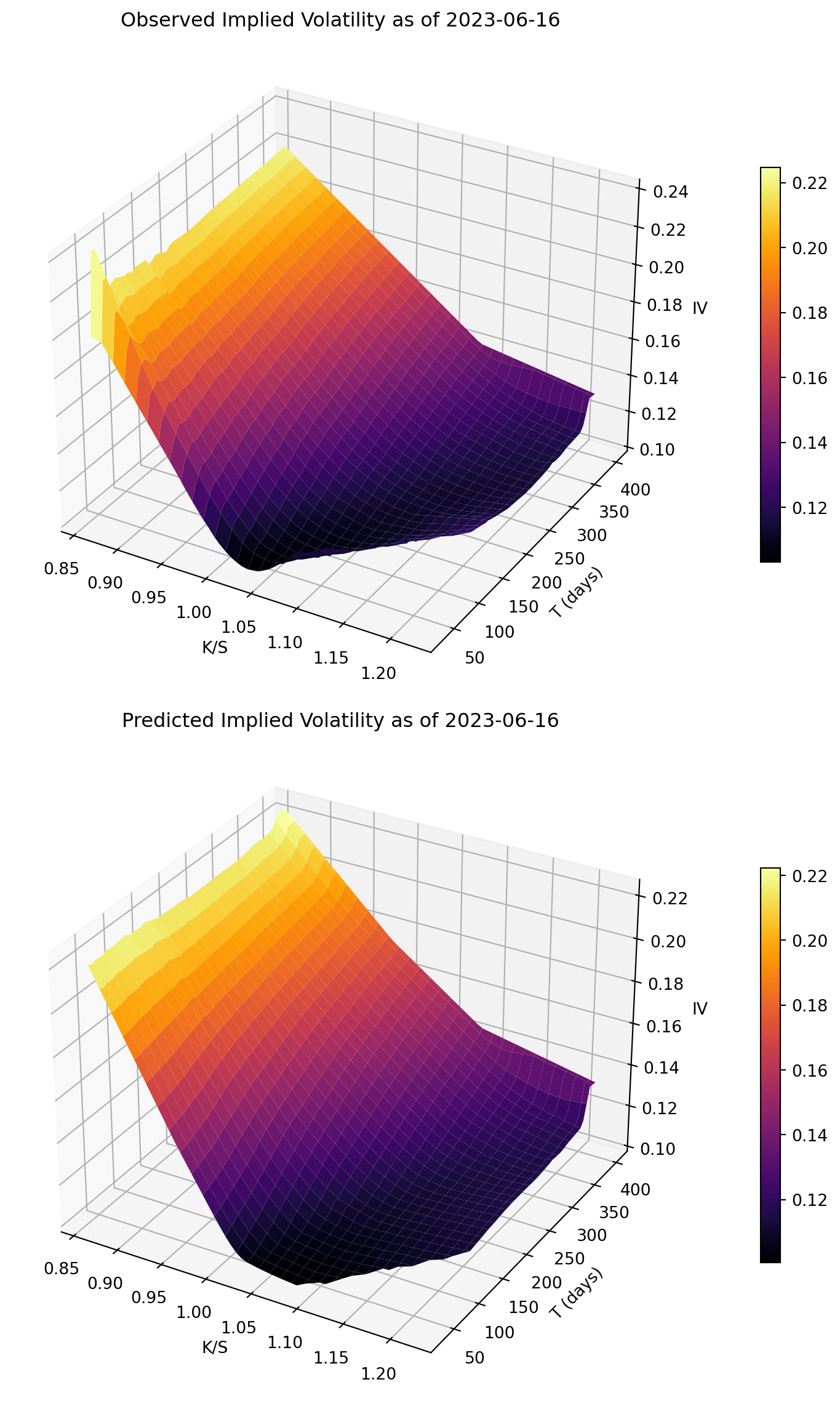
Surface-plot interpretation:
- The objective is shape matching: level, slope, and curvature across moneyness and maturity.
- Good visual agreement supports the idea that the network learned the main surface structure.
Key result:
- The predicted surface broadly reproduces the observed level and shape on the target day.
Takeaways
- This notebook applies the same training/fit/evaluation framework to real options data.
- IV prediction quality should be judged both statistically (MAE/RMSE/R^2) and visually (surface shape).
- Scope note: this is an ML modeling exercise with a random held-out test split, not a trading strategy backtest.