Utility Theory Under Uncertainty
Introduction
In a single period model, agents must decide today how much to consume and how much to save for later. In this note we take that decision as given, and assume that agents derive their utility from consumption at the end of the period, represented as is common in finance by a single good. Agents prefer more to less, but the marginal utility of each additional unit of consumption is decreasing, i.e., the last bite is never as good as the first one.
We capture this intuition by a utility function u: \mathbb{R}^{+} \rightarrow \mathbb{R}, where \mathbb{R}^{+} = [0, \infty) since consumption cannot be negative. We assume throughout that u is continuous, differentiable of all orders, increasing and strictly concave,1 that is, u'(c) > 0 and u''(c) < 0. The level of utility is not important and can even be negative. In some cases it will also be useful to consider utility functions such that u'(0) = \infty, that is, in starvation an extra unit of consumption provides an infinite amount of extra utility.
1 A function f: D \rightarrow \mathbb{R} is concave if f(t x_{1} + (1 - t) x_{2}) \geq t f(x_{1}) + (1 - t) f(x_{2}) for all x_{1}, x_{2} \in D and 0 \leq t \leq 1. The function is strictly concave if the inequality is strict.
2 For small x, y^{x} = \exp(x \ln(y)) \approx 1 + x \ln(y). Taking x = 1 - \gamma and y = c, \begin{aligned} \frac{c^{1 - \gamma} - 1}{1 - \gamma} & \approx \frac{(1 - \gamma) \ln(c)}{1 - \gamma} \\ & = \ln(c). \end{aligned} The error in the approximation is of order (1 - \gamma)^{2}, so it vanishes as \gamma \rightarrow 1 and the limit is exactly \ln(c).
Two families of utility functions will recur throughout these notes. The first is power utility, u(c) = \dfrac{c^{1 - \gamma} - 1}{1 - \gamma}, \quad \gamma > 0, \gamma \neq 1, with marginal utility u'(c) = c^{-\gamma}, together with log utility, u(c) = \ln(c). Log utility is not a separate special case but the \gamma \rightarrow 1 limit of power utility.2
The second family is exponential utility, u(c) = -e^{-ac}, \quad a > 0. We will see that power/log and exponential utility induce different attitudes under uncertainty.
Expected Utility and Risk Aversion
The analysis in the next two sections closely follows Chapter 1 in Ingersoll (1987). Denote by \overset{\sim}{W} the wealth of the agent at the end of the period, a random variable defined over a probability space (\Omega, \operatorname{P}), where the tilde emphasizes that its value is unknown today. Since all wealth is consumed at the end of the single period, \overset{\sim}{W} plays the role of end-of-period consumption, and we use u(\overset{\sim}{W}) interchangeably with u(c) from here on.
Under uncertainty the utility of final consumption is random too, so the agent ranks gambles not by the consumption they deliver but by the expected utility they deliver: U(\overset{\sim}{W}) = \operatorname{E}(u(\overset{\sim}{W})). Thus, we have that \overset{\sim}{W}_{1} \succsim \overset{\sim}{W}_{2} if U(\overset{\sim}{W}_{1}) \geq U(\overset{\sim}{W}_{2}), and \overset{\sim}{W}_{1} \sim \overset{\sim}{W}_{2} if U(\overset{\sim}{W}_{1}) = U(\overset{\sim}{W}_{2}). Note that the expected utility of a certain level of wealth W is just u(W).
Consider now a fair gamble \tilde{\varepsilon}, by which we mean a random variable with \operatorname{E}(\tilde{\varepsilon}) = 0 and \operatorname{V}(\tilde{\varepsilon}) > 0. Adding it to a certain wealth W gives \overset{\sim}{W} = W + \tilde{\varepsilon}, which has the same mean as W but strictly more variance. An agent is risk-averse if she prefers the certain wealth to the gamble, that is, if u(W) > \operatorname{E}(u(W + \tilde{\varepsilon})). \tag{1}
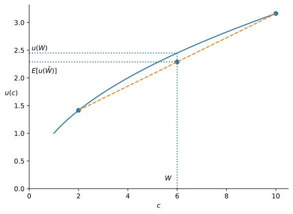
Figure 1 illustrates why this holds for a strictly concave utility function. Take a gamble that pays W - \Delta or W + \Delta with equal probability, so that \operatorname{E}(\overset{\sim}{W}) = W. Expected utility is the height of the chord at W, and concavity places the chord strictly below the curve, so \operatorname{E}(u(\overset{\sim}{W})) < u(W): the sure thing beats the gamble. The figure also marks two quantities defined in the next section, the certainty equivalent CE and the insurance premium \Pi_{i} = W - CE.
The formal statement behind this argument is the following.
Property 1 (Jensen’s Inequality) Let f: D \rightarrow \mathbb{R} be a twice-continuously differentiable and strictly concave function, and X a random variable defined in a probability space (\Omega, \operatorname{P}) such that the range of X is contained in the domain of f, and \operatorname{V}(X) > 0. Then we have that3 f(\operatorname{E}(X)) > \operatorname{E}(f(X)).
3 Let m = \operatorname{E}(X). Since f is strictly concave and differentiable, the tangent line at m lies strictly above the graph of f for all x \neq m: f(x) < f(m) + f'(m)(x - m). Setting x = X and taking expectations, \operatorname{E}(f(X)) < f(m) + f'(m)\,\operatorname{E}(X - m) = f(\operatorname{E}(X)), where \operatorname{E}(X - m) = 0 follows from m = \operatorname{E}(X), and the inequality is strict because \operatorname{V}(X) > 0 ensures X \neq m with positive probability.
Jensen’s inequality shows that strict concavity in u implies risk-aversion. The converse is also true: risk-aversion implies that u must be strictly concave.4
4 Fix any x_{1}, x_{2} in the domain of u and any t \in (0, 1), and let d = x_{1} - x_{2} and W = t x_{1} + (1 - t) x_{2}. Consider the gamble \tilde{\varepsilon} that pays (1 - t) d with probability t and -t d with probability 1 - t. It is fair, since \operatorname{E}(\tilde{\varepsilon}) = 0, and it moves wealth to exactly x_{1} or x_{2}, because W + (1 - t) d = x_{1} and W - t d = x_{2}. A risk-averse investor dislikes it, so \begin{aligned} u(W) & > \operatorname{E}(u(W + \tilde{\varepsilon})) \\ & = t\, u(x_{1}) + (1 - t)\, u(x_{2}), \end{aligned} which, given the definition of W, is exactly strict concavity.
Property 2 (Risk Aversion and Concavity of the Utility Function) An agent is risk-averse as defined in (1) if and only if her utility function is strictly concave.
Strict concavity is therefore the defining mathematical feature of risk-averse preferences. It also lets us ask not just whether an agent is risk-averse but how much so, a comparison we make concrete next by asking what she would pay to get rid of a risk.
Local Risk Aversion
A more concave utility function should induce more risk aversion. We can formalize this intuition by looking at the insurance premium for a gamble with a very small variance.
Let \tilde{\varepsilon} be a fair gamble with \operatorname{V}(\tilde{\varepsilon}) = \sigma_{\varepsilon}^{2}, and expand both sides of (2) around W. To first order on the left, u(W - \Pi_{i}) \approx u(W) - u'(W) \Pi_{i}, \tag{3} and to second order on the right, using \operatorname{E}(\tilde{\varepsilon}) = 0 and \operatorname{E}(\tilde{\varepsilon}^{2}) = \sigma_{\varepsilon}^{2}, \operatorname{E}(u(W + \tilde{\varepsilon})) \approx u(W) + u'(W) \operatorname{E}(\tilde{\varepsilon}) + \frac{1}{2} u''(W) \operatorname{E}(\tilde{\varepsilon}^{2}) = u(W) + \frac{1}{2} u''(W) \sigma^{2}_{\varepsilon}. \tag{4} Equating (3) and (4) gives where \mathit{ARA} is the Arrow-Pratt coefficient of absolute risk-aversion (Ingersoll 1987, sec. 1.12). It is literally the dollar premium the agent pays per unit of variance, so an agent with a higher \mathit{ARA} pays more to shed any given gamble. Since \mathit{ARA} depends on W, we can also ask how risk-aversion changes with wealth: an agent with decreasing absolute risk-aversion (DARA) pays a smaller dollar premium as she gets wealthier, the pattern favored by most empirical evidence and introspection.
The factor of W in the second coefficient appears once we look at proportional rather than dollar gambles. For \tilde{\varepsilon} = W \tilde{\delta}, where \tilde{\delta} is a percentage shock with \operatorname{E}(\tilde{\delta}) = 0 and \operatorname{V}(\tilde{\delta}) = \sigma_{\delta}^{2}, substituting into (5) gives \Pi_{i} \approx \frac{1}{2} \mathit{ARA} \cdot W^{2} \sigma_{\delta}^{2} = \frac{1}{2} \mathit{RRA} \cdot W \sigma_{\delta}^{2}, \qquad \mathit{RRA} = -\frac{u''(W)}{u'(W)} W, where \mathit{RRA} is the coefficient of relative risk-aversion. Dividing by W, the fraction of wealth the agent sacrifices to eliminate the proportional gamble is \Pi_{i} / W \approx \frac{1}{2} \mathit{RRA} \cdot \sigma_{\delta}^{2}. This is why an agent with constant relative risk-aversion (CRRA) keeps the same fraction of wealth in risky assets regardless of how wealthy she is, a portfolio-choice result we state here for intuition and derive formally in a later note.
Example 3 Take u(W) = \frac{W^{1 - \gamma} - 1}{1 - \gamma} Then u'(W) = W^{-\gamma} and u''(W) = -\gamma W^{-\gamma - 1}, implying that \mathit{RRA} = -\left( \frac{-\gamma W^{-\gamma -1}}{W^{-\gamma}}\right) W = \gamma Power utility is an example of a function that exhibits constant relative risk-aversion.
Example 4 For exponential utility u(W) = -e^{-aW} with a > 0, we have u'(W) = a e^{-aW} and u''(W) = -a^{2} e^{-aW}, so \mathit{ARA} = \frac{a^{2} e^{-aW}}{a e^{-aW}} = a. The coefficient of absolute risk-aversion is constant (equal to a) and independent of W. Exponential utility therefore exhibits constant absolute risk-aversion (CARA). A direct implication is that the insurance premium \Pi_{i} \approx \frac{1}{2} a \sigma_{\varepsilon}^{2} does not depend on the agent’s wealth: a billionaire and a middle-class worker with the same CARA parameter a would pay identical dollar amounts to insure against the same gamble. This is analytically convenient but empirically implausible, since most people become less risk-averse in absolute terms as they accumulate wealth.
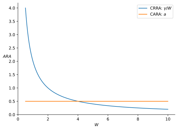
Figure 2 puts these two examples side by side. The power-utility agent’s ARA falls as wealth grows (DARA), while the exponential-utility agent’s ARA stays flat at a no matter how wealthy she becomes (CARA). At low wealth the CRRA agent can be far more risk-averse than the CARA agent; at high wealth the ordering flips, since the CRRA agent’s ARA keeps shrinking while the CARA agent’s does not.
Practice Problems
These problems give you a chance to practice the concepts introduced in this chapter. Try to solve each one on your own before expanding the solution.
Problem 1 (The Insurance Decision Across Wealth Levels) Clara Bennett, a graduate student, has a logarithmic utility function u(W) = \ln W, and her current wealth is \$5{,}000.
- Clara faces a 50/50 chance of either winning or losing \$1{,}000. She can buy insurance for \$125 that would entirely eliminate this risk. Should she buy the insurance or take the gamble?
- Suppose Clara took the gamble in part (a) and lost, which reduced her wealth to \$4{,}000. If she is now offered the same gamble and the same insurance for \$125, should she buy the insurance this time?
Solution
Without insurance, the gamble leaves wealth at \$4{,}000 or \$6{,}000 with equal probability, so \operatorname{E}(u) = 0.5 \ln(4{,}000) + 0.5 \ln(6{,}000) = 8.4968. Buying insurance guarantees \$5{,}000 - \$125 = \$4{,}875, so u(4{,}875) = \ln(4{,}875) = 8.4919. Since 8.4968 > 8.4919, the gamble yields higher expected utility than the insured outcome, so she should take the gamble rather than buy insurance at this price.
After the loss, wealth is \$4{,}000, and the same gamble leaves wealth at \$3{,}000 or \$5{,}000 with equal probability, so \operatorname{E}(u) = 0.5 \ln(3{,}000) + 0.5 \ln(5{,}000) = 8.2618. Buying insurance guarantees \$4{,}000 - \$125 = \$3{,}875, so u(3{,}875) = \ln(3{,}875) = 8.2623. Now 8.2623 > 8.2618, so she should buy the insurance. Nothing about the gamble or its price changed but her wealth fell. This is exactly the decreasing absolute risk-aversion (DARA) property of log utility. Since \mathit{ARA} = 1/W rises as W falls, the same \$1{,}000 gamble looms larger at lower wealth, making the fixed \$125 insurance premium worth paying.
Problem 2 (Maximum Willingness to Pay for Insurance) Ines Kowalski owns Kowalski Woodworks, a furniture workshop that makes up nearly all of her net worth. She faces the following risks: a 10% chance that a fire will reduce her net worth to \$1, a 10% chance that a fire will lower it to \$50{,}000, and an 80% chance that nothing will happen, maintaining the business’s value at \$100{,}000. Her utility function is logarithmic, given by u(W) = \ln W. She is considering an insurance policy that would provide a payout of \$99{,}999 in the first scenario, \$50{,}000 in the second, and nothing in the third. What is the maximum amount she would be willing to pay for this insurance policy?
Solution
The policy fully restores her net worth to \$100{,}000 in every scenario, since \$1 + \$99{,}999 = \$100{,}000, \$50{,}000 + \$50{,}000 = \$100{,}000, and \$100{,}000 + \$0 = \$100{,}000. Paying a premium \Pi therefore leaves her with a certain wealth of \$100{,}000 - \Pi regardless of what happens. Her maximum willingness to pay is the value of \Pi that makes her indifferent between this certain outcome and facing the risk uninsured: \ln(100{,}000 - \Pi) = 0.1 \ln(1) + 0.1 \ln(50{,}000) + 0.8 \ln(100{,}000). The right-hand side is 0.1(0) + 0.1(10.8198) + 0.8(11.5129) = 10.2923, so 100{,}000 - \Pi = \exp(10.2923) = 29{,}505.10, which gives \Pi = 100{,}000 - 29{,}505.10 = \$70{,}494.90.Problem 3 (A Fair Lottery and Concavity) You are offered the possibility to participate at the following lottery:
| Gain | Probability |
|---|---|
| 2 | 0.5 |
| 0 | 0.5 |
The cost of participating at the lottery is 1 unit of consumption. If you choose not to participate, you keep your unit of consumption.
- Is this a fair gamble?
- Show that the decision not to participate at the gamble implies that your utility function is concave.
Solution
The expected gain from playing is 0.5(2) + 0.5(0) = 1, which exactly equals the 1 unit it costs to play. Since the price of the lottery equals its expected payoff, it is an actuarially fair gamble.
Let W denote current wealth, which includes the 1 unit at stake. Not participating leaves wealth at W with certainty. Participating replaces that unit with the lottery, so wealth becomes W + 1 with probability 0.5 (if you win the 2, net of the 1 paid to play) or W - 1 with probability 0.5 (if you win the 0). Note that W = 0.5 (W + 1) + 0.5 (W - 1), so the decision not to participate says u(W) > 0.5\, u(W + 1) + 0.5\, u(W - 1), i.e., u\big(0.5 (W+1) + 0.5(W-1)\big) > 0.5\, u(W+1) + 0.5\, u(W-1). This is exactly the definition of strict concavity evaluated at x_{1} = W+1, x_{2} = W - 1, and t = 0.5. Hence, turning down this fair gamble at every wealth level is equivalent to u being strictly concave, consistent with Property 2.
Problem 4 (Mean-Preserving Spreads and Risk Aversion) Consider gamble A:
| Gain | Probability |
|---|---|
| -2 | 0.09 |
| 4 | 0.30 |
| 10 | 0.40 |
| 16 | 0.21 |
From A, we can construct another gamble B by adding white noise to a number of outcomes. Indeed, we can replace the outcome 4 by the gamble A':
- 3 with probability 1/2
- 5 with probability 1/2
with \operatorname{E}(A') = 4. In the same manner, we can replace outcome 16 with gamble A'':
- 12 with probability 1/3
- 18 with probability 2/3
with \operatorname{E}(A'') = 16.
Show formally why any risk averse individual prefers gamble A to gamble B.
Solution
The outcomes -2 and 10 are shared by both gambles, so they contribute identically to \operatorname{E}(u(A)) and \operatorname{E}(u(B)). The two gambles differ only in how they resolve the 4 and 16 branches, so \operatorname{E}(u(A)) - \operatorname{E}(u(B)) = 0.30 \Big(u(4) - \big[0.5\, u(3) + 0.5\, u(5)\big]\Big) + 0.21 \Big(u(16) - \big[\tfrac{1}{3} u(12) + \tfrac{2}{3} u(18)\big]\Big). By Jensen’s inequality (Property 1), since u is strictly concave and \operatorname{E}(A') = 4 with \operatorname{V}(A') > 0, u(4) = u(\operatorname{E}(A')) > \operatorname{E}(u(A')) = 0.5\, u(3) + 0.5\, u(5). Likewise, since \operatorname{E}(A'') = 16 with \operatorname{V}(A'') > 0, u(16) = u(\operatorname{E}(A'')) > \operatorname{E}(u(A'')) = \tfrac{1}{3} u(12) + \tfrac{2}{3} u(18). Both terms in brackets above are therefore strictly positive, and since they are multiplied by the strictly positive probabilities 0.30 and 0.21, we obtain \operatorname{E}(u(A)) > \operatorname{E}(u(B)). Since A and B have the same mean but B is riskier (it replaces two certain outcomes of A with fair gambles around those same values), every risk-averse individual, regardless of the specific strictly concave u she holds, prefers A to B.Problem 5 (Divergent Beliefs and the Incentive to Litigate) A distant relative in Europe has recently passed away, leaving behind an estimated fortune of \$1{,}000{,}000. This has left two grieving but competing close relatives: Peter, who currently has no wealth, and Paul, who has \$10{,}000. With the will missing, they can pursue legal action, but the winner will incur legal costs amounting to 10% of the inheritance. Both Peter and Paul share the same utility function: U(W) = W^{1/2}. Peter and Paul both agree that Peter has a 60% chance of winning the million, while Paul has a 40% chance. The judge cannot issue a split decision; the entire amount must go to one of them.
- Should Peter and Paul take their dispute to court, or is there a mutually beneficial agreement they could reach instead?
- Does the conclusion change if the heirs disagree on the probabilities? For instance, what if Peter believes he has an 80% chance of winning, while Paul thinks he has an 80% chance of winning?
Solution
Since only the winner bears the legal cost, going to court leaves the winner with \$1{,}000{,}000 - \$100{,}000 = \$900{,}000 on top of her current wealth, while the loser’s wealth is unaffected.
Under the agreed-upon probabilities, Peter’s wealth from litigating is \$900{,}000 with probability 0.6 or \$0 with probability 0.4, so \operatorname{E}(U_{\text{Peter}}) = 0.6 \sqrt{900{,}000} = 180 \sqrt{10} \approx 569.21. Since U(W) = \sqrt{W}, the certainty equivalent is CE = \operatorname{E}(U)^{2}, so CE_{\text{Peter}} = (180\sqrt{10})^{2} = 32{,}400 \times 10 = \$324{,}000. Paul’s wealth from litigating is \$10{,}000 + \$900{,}000 = \$910{,}000 with probability 0.4 or \$10{,}000 with probability 0.6, so \operatorname{E}(U_{\text{Paul}}) = 0.4 \sqrt{910{,}000} + 0.6 \sqrt{10{,}000} = 40 \sqrt{91} + 60 \approx 441.58, CE_{\text{Paul}} = (40\sqrt{91} + 60)^{2} = 149{,}200 + 4{,}800 \sqrt{91} \approx \$194{,}989.08. A settlement that gives Peter a certain share x of the estate and Paul the remaining 1{,}000{,}000 - x (on top of her \$10{,}000) makes both better off than litigating whenever x \geq 324{,}000 and 10{,}000 + (1{,}000{,}000 - x) \geq 194{,}989.08, i.e., x \leq 815{,}010.92. Since 324{,}000 \le 815{,}010.92, a wide range of settlements dominates litigation for both parties. For instance, splitting the estate in proportion to each party’s odds of winning, \$600{,}000 to Peter and \$400{,}000 to Paul, leaves Peter with \$600{,}000 \gg \$324{,}000 and Paul with \$410{,}000 \gg \$194{,}989.08. Litigation is dominated because it is both risky, which risk-averse (concave U) agents dislike, and wasteful, since it burns \$100{,}000 in legal fees that a private settlement avoids entirely. They should settle, not litigate.
Now suppose each heir is optimistic about her own chances and believes she has an 80% chance of winning. Recomputing each party’s certainty equivalent under her own (subjective) probability of winning, \operatorname{E}(U_{\text{Peter}}) = 0.8 \sqrt{900{,}000} = 240\sqrt{10} \approx 758.95, CE_{\text{Peter}} = (240\sqrt{10})^{2} = \$576{,}000. \operatorname{E}(U_{\text{Paul}}) = 0.8 \sqrt{910{,}000} + 0.2 \sqrt{10{,}000} = 80\sqrt{91} + 20 \approx 783.15, CE_{\text{Paul}} = (80\sqrt{91}+20)^{2} = 582{,}800 + 3{,}200\sqrt{91} \approx \$613{,}326.05. For a settlement to beat litigation for both, we would now need Peter’s share x \geq 576{,}000 and Paul’s total wealth 10{,}000 + (1{,}000{,}000-x) \geq 613{,}326.05, i.e., x \leq 396{,}673.95. But 576{,}000 > 396{,}673.95, so no split of the estate satisfies both constraints at once: each heir’s own optimistic belief makes her demand more than the other is willing to concede, and together their demands exceed the entire \$1{,}000{,}000 pie. Even though both parties are risk-averse and litigation is costly, sufficiently divergent beliefs about the probability of winning can eliminate any room for a mutually beneficial settlement and make litigation unavoidable.
Problem 6 (Quadratic Utility and Increasing Risk Aversion) Consider an investor with quadratic utility u(W) = W - \frac{b}{2} W^{2}, \qquad b > 0, \quad W < \frac{1}{b}, where the restriction W < 1/b (the satiation point) is needed to keep u'(W) > 0.
- Derive general expressions for \mathit{ARA}(W) and \mathit{RRA}(W).
- Take b = 0.0001, so satiation occurs at W = \$10{,}000. Compute \mathit{ARA} and \mathit{RRA} at W = \$1{,}000 and again at W = \$4{,}000.
- Is quadratic utility DARA or IARA? Contrast your answer with the log-utility investor of Exercise 1, whose willingness to insure the same \$1{,}000 gamble increased once her wealth fell from \$5{,}000 to \$4{,}000.
Solution
Differentiating, u'(W) = 1 - bW and u''(W) = -b, so \mathit{ARA}(W) = -\frac{u''(W)}{u'(W)} = \frac{b}{1 - bW}, \qquad \mathit{RRA}(W) = \mathit{ARA}(W) \cdot W = \frac{bW}{1 - bW}.
At W = 1{,}000, 1 - bW = 1 - 0.1 = 0.9, so \mathit{ARA}(1{,}000) = \frac{0.0001}{0.9} \approx 0.00011111, \qquad \mathit{RRA}(1{,}000) \approx 0.1111. At W = 4{,}000, 1 - bW = 1 - 0.4 = 0.6, so \mathit{ARA}(4{,}000) = \frac{0.0001}{0.6} \approx 0.00016667, \qquad \mathit{RRA}(4{,}000) \approx 0.6667.
\mathit{ARA} rises by 50%, from about 0.00011 at W = \$1{,}000 to about 0.00017 at W = \$4{,}000, and \mathit{RRA} rises roughly sixfold over the same range. Quadratic utility therefore exhibits increasing absolute risk aversion (IARA): the wealthier this investor becomes, the more dollars she demands to shed a given fixed-dollar risk. This is the opposite of the log-utility investor in Exercise 1, whose \mathit{ARA} = 1/W is DARA and so is higher at lower wealth. IARA is empirically implausible, since wealthier agents should tolerate a fixed-dollar risk better, not worse, and this is the classic objection to quadratic utility.
Problem 7 (How Good Is the Local Approximation?) Marco Delgado has log utility u(W) = \ln W and wealth W = \$100{,}000. His employer offers him a bonus scheme that adds or subtracts \$10{,}000 from his pay with equal probability.
- Compute the exact insurance premium Marco would pay to eliminate this risk.
- Compute the approximation in (5) and compare it with the exact premium.
Solution
By (2), \ln(W - \Pi_{i}) = 0.5 \ln(90{,}000) + 0.5 \ln(110{,}000), so W - \Pi_{i} = \sqrt{90{,}000 \times 110{,}000} \approx \$99{,}498.74, \qquad \Pi_{i} \approx \$501.26.
For log utility \mathit{ARA} = 1/W = 0.00001, and the gamble has variance 10{,}000^{2} = 10^{8}, so \Pi_{i} \approx \frac{1}{2} \times 0.00001 \times 10^{8} = \$500. The approximation misses by about \$1.26, a quarter of a percent, because the gamble is small relative to Marco’s wealth.
Solution
The proportional gamble has \sigma_{\delta}^{2} = 0.01, and power utility has \mathit{RRA} = \gamma, so the fraction of wealth paid is about \frac{1}{2} \gamma \sigma_{\delta}^{2}. For Nadia that is \frac{1}{2} \times 2 \times 0.01 = 1\%, or \$5{,}000; for Owen it is \frac{1}{2} \times 5 \times 0.01 = 2.5\%, or \$1{,}250.
No. Premiums rank risk aversion only for agents who face the same gamble at the same wealth. Nadia’s gamble is ten times larger in dollars, which is why she pays more.
Owen is more risk averse on both measures. His \mathit{RRA} is 5 against Nadia’s 2, and his \mathit{ARA} is 5/50{,}000 = 0.0001 against her 2/500{,}000 = 0.000004.
Problem 9 (Compensation for Taking a Risk) A startup asks Yusuf Adeyemi to invest in a venture whose outcome will add or subtract \$20{,}000 from his wealth with equal probability. Yusuf has exponential utility u(W) = -e^{-aW} with a = 0.00005.
- Use (6) to find the compensatory risk premium, the expected gain the startup must add to the venture for Yusuf to accept it.
- Compare the exact premium with the local approximation.
- Show that, for exponential utility, the answer does not depend on Yusuf’s wealth, and that the insurance premium for the same gamble is exactly the same.
Solution
With exponential utility, (6) becomes e^{-aW} = e^{-a(W + \Pi_{c})} \operatorname{E}\big(e^{-a \tilde{\varepsilon}}\big), so \Pi_{c} = \frac{1}{a} \ln \operatorname{E}\big(e^{-a \tilde{\varepsilon}}\big) = \frac{1}{a} \ln\left(\frac{e^{-1} + e^{1}}{2}\right) = 20{,}000 \times 0.4338 \approx \$8{,}676, using a \times 20{,}000 = 1.
The approximation gives \frac{1}{2} \times 0.00005 \times 20{,}000^{2} = \$10{,}000, about 15\% too high. Here the gamble is large relative to 1/a = \$20{,}000, so the second-order expansion is no longer accurate.
Wealth W cancels from both sides of the equation in part (a), so \Pi_{c} is the same at every wealth level. For the insurance premium, (2) gives e^{-a(W - \Pi_{i})} = e^{-aW} \operatorname{E}\big(e^{-a \tilde{\varepsilon}}\big), which yields the same expression, so \Pi_{i} = \Pi_{c} \approx \$8{,}676. Under constant absolute risk aversion, the two premiums coincide exactly, not just for small gambles.